CHISQN2
Updated: 28 February 2011
Use the aggregate CHISQN2 to calculate the chi-square (χ2) statistic for normalized tables. This function calculates the chi-square statistic by finding the difference between each observed and theoretical frequency for each possible outcome, squaring them, dividing each by the theoretical frequency, and taking the sum of the results. A second important part of determining the test statistic is to define the degrees of freedom of the test: this is essentially the number of squares errors involving the observed frequencies adjusted for the effect of using some of those observations to define the expected frequencies.
CHISQN2 requires the expected results as input to the function.
The value of the chi-square statistic is:
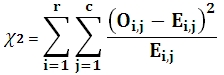
Where
r is the number of rows
c is the number of columns
O is the Observed result
E is the Expected result
Syntax
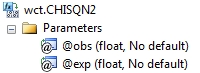
Arguments
@Obs
the observed value. @Obs is an expression of type float or of a type that can be implicitly converted to float.
@Exp
the observed value. @Exp is an expression of type float or of a type that can be implicitly converted to float.
Return Types
float
Remarks
· CHISQN2 is designed for normalized tables.
· CHISQN2 requires the expected values as input. If you want the expected values to be calculated automatically, use the CHISQN function.
· CHISQN2 is an aggregate function and follows the same conventions as all other aggregate functions in SQL Server.
· If you have previously used the CHISQN2 scalar function, the CHISQN2 aggregate has a different syntax. The CHISQN2 scalar function is no longer available in XLeratorDB/statistics2008, though you can still use the scalar CHISQN2_q.
Examples
In this hypothetical situation, we want to determine if there is an association between population density and the preference for a sport from among baseball, football, and basketball. We will use the CHISQ function to calculate the chi-squares statistic.
SELECT wct.CHISQN2(
observed --@obs
,expected --@exp
) as CHISQ
FROM (VALUES
('Basketball', 'Rural', 28, 42.77),
('Basketball', 'Suburban', 35, 38.49),
('Basketball', 'Urban', 54, 35.74),
('Baseball', 'Rural', 60, 50.44),
('Baseball', 'Suburban', 43, 45.4),
('Baseball', 'Urban', 35, 42.16),
('Football', 'Rural', 52, 46.79),
('Football', 'Suburban', 48, 42.11),
('Football', 'Urban', 28, 39.1)
) n(sport, locale, observed, expected)
This produces the following result
CHISQ
----------------------
22.4562079299414
(1 row(s) affected)
What if the expected results and the observed results are in 2 different tables? You could try something likes this.
SELECT * INTO #o
FROM (VALUES
('Basketball', 'Rural', 28),
('Basketball', 'Suburban', 35),
('Basketball', 'Urban', 54),
('Baseball', 'Rural', 60),
('Baseball', 'Suburban', 43),
('Baseball', 'Urban', 35),
('Football', 'Rural', 52),
('Football', 'Suburban', 48),
('Football', 'Urban', 28)
) o(sport, locale, result)
SELECT * INTO #e
FROM (VALUES
('Basketball', 'Rural', 42.77),
('Basketball', 'Suburban', 38.49),
('Basketball', 'Urban', 35.74),
('Baseball', 'Rural', 50.44),
('Baseball', 'Suburban', 45.4),
('Baseball', 'Urban', 42.16),
('Football', 'Rural', 46.79),
('Football', 'Suburban', 42.11),
('Football', 'Urban', 39.1)
)e(sport, locale, result)
SELECT wct.CHISQN2(#o.result, #e.result) as CHISQ
FROM #o, #e
WHERE #o.sport = #e.sport
AND #o.locale = #e.locale
DROP TABLE #o
DROP TABLE #e
This produces the following result.
CHISQ
----------------------
22.4562079299414
(1 row(s) affected)
The previous example relied on the temporary tables. If you want to avoid using temporary tables, you could use the following SQL which uses a CTE and a derived table.
;with obs as (
SELECT *
FROM (VALUES
('Basketball', 'Rural', 28),
('Basketball', 'Suburban', 35),
('Basketball', 'Urban', 54),
('Baseball', 'Rural', 60),
('Baseball', 'Suburban', 43),
('Baseball', 'Urban', 35),
('Football', 'Rural', 52),
('Football', 'Suburban', 48),
('Football', 'Urban', 28)
) o(sport, locale, result)
) SELECT wct.CHISQN2(obs.result, e.result) as CHISQ
FROM (VALUES
('Basketball', 'Rural', 42.77),
('Basketball', 'Suburban', 38.49),
('Basketball', 'Urban', 35.74),
('Baseball', 'Rural', 50.44),
('Baseball', 'Suburban', 45.4),
('Baseball', 'Urban', 42.16),
('Football', 'Rural', 46.79),
('Football', 'Suburban', 42.11),
('Football', 'Urban', 39.1)
)e(sport, locale, result), obs
WHERE obs.sport = e.sport
AND obs.locale = e.locale
This produces the following result.
CHISQ
----------------------
22.4562079299414
(1 row(s) affected)
You could also use 2 derived table, using a CROSS JOIN, but we would recommend not doing this as it will create the Cartesian product of the observed results and the expected results.
SELECT wct.CHISQN2(o_result, e_result) as CHISQ
FROM (VALUES
('Basketball', 'Rural', 28),
('Basketball', 'Suburban', 35),
('Basketball', 'Urban', 54),
('Baseball', 'Rural', 60),
('Baseball', 'Suburban', 43),
('Baseball', 'Urban', 35),
('Football', 'Rural', 52),
('Football', 'Suburban', 48),
('Football', 'Urban', 28)
) o(o_sport, o_locale, o_result)
CROSS JOIN
(VALUES
('Basketball', 'Rural', 42.77),
('Basketball', 'Suburban', 38.49),
('Basketball', 'Urban', 35.74),
('Baseball', 'Rural', 50.44),
('Baseball', 'Suburban', 45.4),
('Baseball', 'Urban', 42.16),
('Football', 'Rural', 46.79),
('Football', 'Suburban', 42.11),
('Football', 'Urban', 39.1)
) e(e_sport, e_locale, e_result)
WHERE e_sport = o_sport
AND e_locale = o_locale
This produces the following result.
CHISQ
----------------------
22.4562079299414
(1 row(s) affected)
What if the expected and observed results are presented in spreadsheet format? We could try the following SQL.
SELECT wct.CHISQN2(o_result, e_result) as CHISQ
FROM (VALUES
('Basketball', 28, 35, 54, 42.77, 38.49, 35.74),
('Baseball', 60, 43, 35, 50.44, 45.4, 42.16),
('Football', 52, 48, 28, 46.79, 42.11, 39.1)
) n(sport, o_rural, o_suburban, o_urban, e_rural, e_suburban, e_urban)
CROSS APPLY(VALUES
('rural', o_rural),
('suburban', o_suburban),
('urban',o_urban)
) o(o_locale, o_result)
CROSS APPLY(VALUES
('rural', e_rural),
('suburban', e_suburban),
('urban',e_urban)
) e(e_locale, e_result)
WHERE o_locale = e_locale
This produces the following result.
CHISQ
----------------------
22.4562079299414
(1 row(s) affected)
In this example, the data are compiled by region in spreadsheet format. We can calculate the chi square statistic for each region in the following SQL.
select n.region
,wct.CHISQN2(o_result, e_result) as CHISQ
from (values
('Midwest','Baseball',2,5,60,17.18,21.12,28.69),
('Midwest','Basketball',49,71,32,38.98,47.92,65.09),
('Midwest','Football',58,58,90,52.83,64.95,88.22),
('Northeast','Baseball',52,69,94,96.62,72.34,119.89),
('Northeast','Basketball',60,36,54,67.41,50.47,83.65),
('Northeast','Football',79,38,89,92.58,69.31,114.88),
('Southeast','Baseball',22,44,28,36.05,26.54,28.97),
('Southeast','Basketball',51,38,45,51.39,37.84,41.3),
('Southeast','Football',90,38,58,71.34,52.52,57.33),
('Southwest','Baseball',26,83,50,35.92,78.19,38.16),
('Southwest','Basketball',23,39,13,16.94,36.88,18),
('Southwest','Football',47,87,39,39.08,85.08,41.52),
('West','Baseball',100,29,80,103.27,32.46,77.21),
('West','Basketball',37,19,4,29.65,9.32,22.16),
('West','Football',73,18,73,81.04,25.47,60.58)
) n(region, sport, o_urban, o_rural, o_suburban, e_urban, e_rural, e_suburban)
CROSS APPLY(VALUES
('rural', o_rural),
('suburban', o_suburban),
('urban',o_urban)
) o(o_locale, o_result)
CROSS APPLY(VALUES
('rural', e_rural),
('suburban', e_suburban),
('urban',e_urban)
) e(e_locale, e_result)
WHERE o_locale = e_locale
GROUP BY n.region
This produces the following result.
region CHISQ
--------- ----------------------
Midwest 91.685259630373
Northeast 63.7898329548442
Southeast 26.2327936119247
Southwest 12.1890926571873
West 32.8659293399746
(5 row(s) affected)
Since the data are compiled in spreadsheet format, we could have also used the scalar function, CHISQ2. The CHISQ2 scalar function does not have addressability to a derived table or a CTE, so the data need to be contained in a table or a temporary table. Here’s the same data put into a temporary table and select using the CHISQ2 function.
SELECT *
INTO #c
FROM (VALUES
('Midwest','Baseball',2,5,60,17.18,21.12,28.69),
('Midwest','Basketball',49,71,32,38.98,47.92,65.09),
('Midwest','Football',58,58,90,52.83,64.95,88.22),
('Northeast','Baseball',52,69,94,96.62,72.34,119.89),
('Northeast','Basketball',60,36,54,67.41,50.47,83.65),
('Northeast','Football',79,38,89,92.58,69.31,114.88),
('Southeast','Baseball',22,44,28,36.05,26.54,28.97),
('Southeast','Basketball',51,38,45,51.39,37.84,41.3),
('Southeast','Football',90,38,58,71.34,52.52,57.33),
('Southwest','Baseball',26,83,50,35.92,78.19,38.16),
('Southwest','Basketball',23,39,13,16.94,36.88,18),
('Southwest','Football',47,87,39,39.08,85.08,41.52),
('West','Baseball',100,29,80,103.27,32.46,77.21),
('West','Basketball',37,19,4,29.65,9.32,22.16),
('West','Football',73,18,73,81.04,25.47,60.58)
) n(region, sport, o_urban, o_rural, o_suburban, e_urban, e_rural, e_suburban)
SELECT region
,wct.CHISQ2('#c'
,'o_urban, o_rural, o_suburban'
,'region'
,region
,'#c'
,'e_urban, e_rural, e_suburban'
,'region'
,region) as CHISQ
FROM #c
GROUP BY region
DROP TABLE #c
This produces the following result.
region CHISQ
--------- ----------------------
Midwest 91.685259630373
Northeast 63.7898329548442
Southeast 26.2327936119247
Southwest 12.1890926571873
West 32.8659293399746
(5 row(s) affected)