KMEANS
Updated: 31 July 2015
Use the table-valued function KMEANS to perform k-means clustering in N-dimensions. The clustering algorithm minimizes the Euclidean distance among the cluster means and the supplied points.
The default solution for the KMEANS function uses an Expectation / Maximization (EM) scheme to assign the data points to a cluster. As such, it always returns a solution, but can be computationally intensive. Alternatively, you can specify other clustering algorithms which are computationally more efficient but may not return a solution. See the algorithm section of this document.
The KMEANS function allows you to specify the starting point for the clusters or you can specify that the function should randomly choose the clusters from the supplied data. If the clusters are to be randomly generated, you also have the ability to specify the number of times to generate clusters and KMEANS will return the best solution.
Given the data points and the clusters, the KMEANS EM process consists of calculating the Euclidean distance between each row of data and each cluster and assigning the row to the cluster with the smallest (i.e. minimum) distance. It then calculates the mean of all the data points assigned to a cluster and recalculate the Euclidean distance and re-assigns data points to different clusters as required. This process repeats until there are no changes in the assignment process.
The function then returns a variety of information. First, it will return the cluster that each row of data has been assigned to. In order to link the cluster assignment back to the supplied data, you need to provide a unique identifier for each input row. This unique identifier and the cluster assignment are returned by the function.
Second, KMEANS will return the calculated cluster means. These means will be returned in 3rd normal form, consisting of zero-based row and column identifiers. The row identifier links to the cluster number returned to the by the assignment process. The column identifier corresponds to the number of dimensions in the data; in other words if the input data being clustered contained 2 columns the column identifiers would be 0 and 1. If it contained 3 columns, the column identifiers would be 0, 1, and 2.
Third, KMEANS returns a count of the number of data rows assigned to the each cluster.
Fourth, KMEANS returns the within sum-of squares for each cluster. This is simply the sum of the Euclidean distance for all the data points in a cluster.
Fifth, KMEANS returns the total within sum-of-squares which is the sum of the within sum-squares.
Sixth, KMEANS return the total sum-of squares for all the columns in the data points.
Seventh, KMEANS return the between sum-of-squares as the difference between the total sum-of-squares and the total within sum-of-squares.
Finally, KMEANS returns the number of iterations actually used to return the solution.
Syntax
SELECT * FROM [wct].[KMEANS](
<@dataQuery, nvarchar(max),>
,<@meansQuery, nvarchar(max),>
,<@numclusters, int,>
,<@nstart, int,>
,<@algorithm, nvarchar(4000),>
,<@itermax, int,>
,<@seed, int,>
,<@Formula, nvarchar(max),>)
@dataQuery
the SELECT statement, as a string, which, when executed, creates the resultant table of data points used in the calculation. The first column should contain a unique row identifier so that the data points can be linked to the cluster.
@meanQuery
the SELECT statement, as a string, which, when executed, creates the resultant table of clusters used in the calculation. If you want the function to randomly select clusters from the data points simply enter a NULL.
@numclusters
the number of clusters to assign the data points to. @numclusters is not used if @meansQuery is not NULL. @numclusters is of type int or of a type that implicitly converts to int.
@nstart
The number of times to generate clusters and calculate the k-means. @nstart is not used if @meansQuery is not NULL. @nstart is of type int or of a type that implicitly converts to int.
@algorithm
The algorithm used to calculate the cluster means. Use 'EM' for the method described in [1]. Use 'HartiganWong' for the Method described in [2]. Use 'Lloyd' for the method described in [3]. Use 'MacQueen' for the method described in [4].
@itermax
The maximum number of iterations to be used if @algorithm is not 'EM'.
@seed
an optional integer value to be passed in as a seed value to the random number generator. @seed is only used if @meansQuery is NULL to support the reproducibility of the result. @seed must be of type int or of a type that implicitly converts to int.
@Formula
a string identifying the distance calculation method. Only squared Euclidean distance is supported at this time.
Return Types
RETURNS TABLE (
[label] [nvarchar](15) NULL,
[rowid] [sql_variant] NULL,
[colid] [sql_variant] NULL,
[val] [float] NULL
)
Table Description
label
Identifies the value being returned:
|
assign
|
cluster assigned to the input row.
|
|
means
|
average of all the data points assigned to a cluster
|
|
count
|
number of input rows assigned to each cluster
|
|
withinss
|
within sum-of-square for each cluster
|
|
tot_withinss
|
total within sum-of-squares
|
|
betweenss
|
between sum-of-squares
|
For more information on how these statistics are calculated see the Examples.
rowid
a row identifier. When label = 'assign' the row identifier is the unique identifier passed into the function as part of @dataQuery. When label = 'means', 'count', or withinss the rowid is the cluster number of the means. For all other returned values the rowid is zero.
colid
a column identifier. colid is only meaningful when label = 'means'.
val
the value associated with the label, rowid, and colid.
Remarks
· If the number of rows returned by @meansQuery is greater than the number of rows returned by @dataQuery, then no rows are returned by the function.
Examples
Example #1
In this example we create 100 x- and y- data points. This first 50 have their co-ordinates generated from a random normal distribution with mean 0 and standard deviation of 0.5. The next 50 from a random normal distribution with mean 1 and standard deviation of 0.5. We want to cluster into 2 groups. We store the data points in #a and the KMEANS results in #cl.
SELECT
*
INTO
#a
FROM (VALUES
(1,-0.288734000529778,0.028008366637481)
,(2,1.00124136514641,-0.0259909530904495)
,(3,0.0333504354650915,-0.876618679571135)
,(4,0.933425922353431,0.0496637970439137)
,(5,-0.675451343015356,-0.285925028947782)
,(6,0.0104917931771187,-0.487004791402046)
,(7,0.624957285484608,-0.0899531155237702)
,(8,-0.357621093611398,0.507471586371829)
,(9,-0.376344484108871,-0.996374244344291)
,(10,-0.469269351803447,-0.213639643602714)
,(11,-0.526256639669368,0.0583186417913532)
,(12,-0.218579766590199,-0.446603785027476)
,(13,0.165589586479491,0.166951471249613)
,(14,-1.00710524896036,0.205714960307865)
,(15,0.105990216686146,-0.0165180796379959)
,(16,0.618337523208285,-1.23294909688001)
,(17,1.01878700912022,1.28572907293332)
,(18,0.650587996100294,-0.1026496287341)
,(19,0.378387381897981,0.325596640793835)
,(20,-0.863365199557165,0.136883245518274)
,(21,-0.300753354003391,0.512336617409175)
,(22,-0.176023228291308,0.408829723187044)
,(23,0.351761951378447,-0.104896585614254)
,(24,-0.0528356670018872,0.189083886104254)
,(25,-0.629324314030086,-0.472704415561946)
,(26,0.842217854047057,0.428461505449659)
,(27,0.455695645897981,-0.230519169442177)
,(28,0.118715136245513,1.20838667689411)
,(29,0.609054305162906,-0.825524447844094)
,(30,-0.669387143617486,-0.231993621483007)
,(31,0.3304101488949,0.412689931379621)
,(32,-0.261456188156711,0.255066273439332)
,(33,0.341872760925356,-0.2947405192575)
,(34,-0.0304109773300371,-0.498390371103761)
,(35,0.316480356515725,0.0722378523553483)
,(36,0.667758807529696,-0.00715370658345669)
,(37,0.0036450451584494,-0.89514061863203)
,(38,0.508779318476046,0.0172755335669255)
,(39,-0.594217017573989,0.0951151578462286)
,(40,-0.360802220218008,0.0873631984909208)
,(41,0.759608855694089,-0.527508521301341)
,(42,0.188693986511965,0.238066639151315)
,(43,-1.02611141021686,0.68928506847962)
,(44,-0.682018726041188,0.228118201589906)
,(45,-0.100390507794561,-0.567794235187172)
,(46,0.432889702167244,-0.217822734845953)
,(47,-0.0509416278576112,0.173051809776803)
,(48,0.312093736010326,-0.323522815659134)
,(49,0.479502688893913,-1.07882316750764)
,(50,0.83552741443147,0.442125410014104)
,(51,0.585261194187741,0.900055085949283)
,(52,0.713219864615859,0.677443021570104)
,(53,1.75195030450227,1.08266051062103)
,(54,0.612927535197297,1.21940935035723)
,(55,1.42286577009465,1.44165140997435)
,(56,0.369658560590612,-0.0261684919509764)
,(57,0.822728798463011,0.181810365970488)
,(58,0.963221990431761,1.71520117059409)
,(59,0.415674287787822,1.52331442355577)
,(60,0.682625867545545,1.21764447445384)
,(61,0.985579223535843,1.35758920355553)
,(62,1.33534798436697,1.4585874588205)
,(63,0.174726728287445,-0.33046139923284)
,(64,0.825122880394366,1.55513854831941)
,(65,1.37820321927274,0.757506201718838)
,(66,0.730595420011204,1.1153084153156)
,(67,1.11364596083647,0.852421099558211)
,(68,1.24611428503222,1.43598247703937)
,(69,1.13391750766584,0.825763775522194)
,(70,1.32662883973569,1.25925188294412)
,(71,0.93864566951131,0.804657510680511)
,(72,0.79316174320394,0.453606395449247)
,(73,-0.321574476014489,1.60500525522013)
,(74,0.953529490760264,1.37045000563714)
,(75,1.21514234817999,1.86213111957823)
,(76,1.26769942043408,1.03257696628965)
,(77,0.722360824343374,1.56250137291409)
,(78,1.88975145488757,1.98770952700954)
,(79,1.14321220981441,0.859258942480517)
,(80,1.06315792922944,0.338524443622392)
,(81,1.63613338973426,0.880324216430942)
,(82,0.64076688934037,0.892979380007308)
,(83,0.774830688037644,1.07584025225466)
,(84,2.19872624002488,1.85615248865964)
,(85,1.00556459361044,0.836928053747326)
,(86,1.81678421070415,1.18650232790246)
,(87,0.280746677542739,0.886157967552234)
,(88,0.904741598978549,1.01022535426252)
,(89,1.18921195181842,1.15702883175313)
,(90,1.1500192726029,1.66410734801849)
,(91,0.497181870244582,1.06065918874539)
,(92,1.00962963731269,1.35642116001556)
,(93,0.461289673444009,1.38943001489177)
,(94,1.35635166262214,1.45738663542782)
,(95,1.54238754493032,0.712802723907808)
,(96,-0.112493848243706,1.81344060709734)
,(97,1.61784673115007,0.809521630352994)
,(98,0.379477751595754,0.947107916175124)
,(99,1.22738463449132,1.70202513385709)
,(100,1.3299513190713,1.64704195307279)
)n(r,x,y)
--Run KMEANS and store in #cl
SELECT
*
INTO
#cl
FROM
wct.KMEANS(
'SELECT * FROM #a', --@dataQuery
NULL, --@meansQuery
2, --@numclusters
1, --@nstart
NULL, --@algorithm
NULL, --@itermax
NULL, --@seed
NULL --@formula
)
We can run the following SQL to get the x- and y- data points and their assigned cluster.
--Get the data points and the assigned cluster.
SELECT
#a.r
,#a.x
,#a.y
,#cl.val as cluster
FROM
#a
INNER JOIN
#cl
ON
#a.r = #cl.rowid
WHERE
#cl.label = 'assign'
ORDER BY
r
This produces the following result.
If we take these results and put them in a scatter plot in Excel it would look like this.
The following SQL returns the cluster means.
--Get the cluster means
SELECT
cast(rowid as int) as cluster
,[0] as x
,[1] as y
FROM (
SELECT
rowid
,cast(colid as int) as colid
,val
FROM
#cl
WHERE
label = 'means'
)d
PIVOT(
SUM(val)
FOR colid in([0],[1])
)pvt
ORDER BY
1
This produces the following result
We can add the means to the scatter plot.
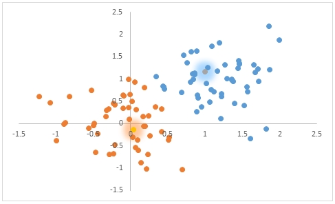
This SQL returns the rest of the statistics from #cl.
SELECT
label
,cast(rowid as int) as rowid
,val
FROM
#cl
WHERE
label <> 'means'
AND label <> 'assign'
This produces the following result.
Example #2
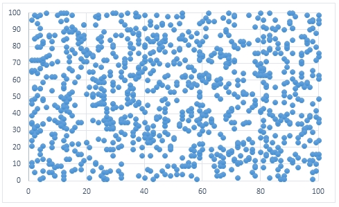
To create some data for this example, we create 1,000 data points consisting of 2 columns which contain uniformly randomly generated integer values between 1 and 100.
SELECT
seq,
seriesValue as x,
wct.RANDBETWEEN(1,100) as y
INTO
#a
FROM
wct.SeriesInt(1,100,NULL,1000,'R')
If we were to create a scatter plot of the input data using EXCEL it would look something like this.
In this example, we will pass 9 starting values into the function.
SELECT
*
INTO
#m
FROM (VALUES
(25,25),(25,50),(25,75),
(50,25),(50,50),(50,75),
(75,25),(75,50),(75,75)
)n(x,y)
A scatter plot of the starting points would look like this.
We will pass this data into the function and store the results in the #cl temp table.
SELECT
*
INTO
#cl
FROM
wct.KMEANS(
'SELECT * FROM #a', --@dataQuery
'SELECT * FROM #m', --@meansQuery
NULL, --@numclusters
NULL, --@nstart
NULL, --@algorithm
NULL, --@itermax
NULL, --@seed
NULL --@formula
)
We can extract the means (clusters) from the #cl table with the following SQL, which will also PIVOT the result into 2 columns. Your results will be different.
SELECT cast(rowid as int) as rowid, [0],[1]
FROM (
SELECT rowid,cast(colid as int) as colid,val
FROM #cl
WHERE label = 'means'
)d
PIVOT(SUM(val) FOR colid in([0],[1]))pvt
ORDER BY rowid
This produces the following result.
We have 9 means (clusters), numbered 0 through 8 and each cluster contains 2 columns, 0 and 1. We are able to identify the entries in the #cl table because they have the label 'means'.
The following scatter plot shows the original clusters (the blue circles) passed into the function and the values calculated by the function (the orange triangles).
The means are simply the column averages of the input data grouped by the cluster to which the input data have been assigned. These could be manually calculated (though there is no reason to as they are already returned by the function) with the following SQL.
SELECT
#cl.val,
AVG(cast(#a.x as float)) as x,
AVG(cast(#a.y as float)) as y
FROM
#a
INNER JOIN
#cl
ON
#a.seq = #cl.rowid
WHERE
#cl.label = 'assign'
GROUP BY
#cl.val
ORDER BY
1
The following SQL demonstrates how to link the original data points to their assigned cluster.
--Get the data points and the assigned cluster.
SELECT TOP 20 #a.seq,#a.x,#a.y,#cl.val as cluster
FROM #a
INNER JOIN #cl
ON #a.seq = #cl.rowid
WHERE #cl.label = 'assign'
ORDER BY seq
This produces the following result. Your results will be different.
In this scatter plot we have returned all thousand rows and created an Excel scatter plot showing the clustering for all the data points.
KMEANS returns the count of clusters for each mean. You can get this from the temp table with the following SQL.
--Get the cluster count for each mean
SELECT cast(rowid as int) as cluster, val as [cluster count]
FROM #cl
WHERE label = 'count'
ORDER BY 1
This produces the following result.
You could get the same result with the following SQL.
--Manually calculate the cluster count
SELECT val as cluster, COUNT(*) as [cluster count]
FROM #cl
WHERE label = 'assign'
GROUP BY val
ORDER BY 1
You can get the within sum-of-squares from the temp table with the following SQL.
--Get the within sum-of-squares
SELECT cast(rowid as int) as cluster, val as withinss
FROM #cl
WHERE label = 'withinss'
This produces the following result.
The within sum-squares is the sum of the Euclidean distance from each data point to its assigned mean. The following SQL replicates the within sum-of-squares values returned by the function.
--Manually calculate the within sum-of squares
;with mycte as (
SELECT rowid as rowid,[0] as x,[1] as y
FROM (
SELECT cast(rowid as int) as rowid, cast(colid as int) as colid, val
FROM #cl
WHERE label = 'means'
)d
PIVOT(sum(val) for colid in([0],[1]))pvt
)
SELECT #cl.val, SUM(POWER(#a.x-m.x,2)+POWER(#a.y-m.y,2)) as withinss
FROM #cl
INNER JOIN #a
ON #cl.rowid = #a.seq
INNER JOIN mycte m
ON #cl.val = m.rowid
WHERE #cl.label = 'assign'
GROUP BY #cl.val
The total within sum-of-squares is the sum of the within sum-of-squares. This can be obtain directly from the temp table.
SELECT val as [total withinss]
FROM #cl
WHERE label = 'tot_withinss'
This produces the following result.
The following SQL demonstrates the logic behind the calculation of the total within sum-of-squares.
--Manually calculate the total within sum-of-squares
;with mycte as (
SELECT rowid as rowid,[0] as x,[1] as y
FROM (
SELECT cast(rowid as int) as rowid, cast(colid as int) as colid, val
FROM #cl
WHERE label = 'means'
)d
PIVOT(sum(val) for colid in([0],[1]))pvt
)
SELECT SUM(POWER(#a.x-m.x,2)+POWER(#a.y-m.y,2)) as [total withinss]
FROM #cl
INNER JOIN #a
ON #cl.rowid = #a.seq
INNER JOIN mycte m
ON #cl.val = m.rowid
WHERE #cl.label = 'assign'
The following SQL obtains the total sum-squares.
--Get the total sum-of-squares
SELECT val as totss
FROM #cl
WHERE label = 'totss'
This produces the following result.
The following SQL demonstrates the logic behind the calculation of the total sum-of-squares.
--Manually calculate the total sum-of-squares
SELECT (sx+sy)*n as totss
FROM (
SELECT VARP(x) as sx, VARP(y) as sy, COUNT(*) as n
FROM #a
)b
The between sum-of-squares is simply the difference between the total sum-of-squares and the total within sum-of squares. You can obtain between sum-of-squares from the temp table with the following SQL.
--Get the between sum-of-squares
SELECT val as betweenss
FROM #cl
WHERE label = 'betweenss'
This produces the following result.
Example #3: Cluster starting points are randomly chosen from the supplied data points
SELECT
seq,
seriesValue as x,
wct.RANDBETWEEN(1,100) as y
INTO
#a
FROM
wct.SeriesInt(1,100,NULL,1000,'R')
SELECT
*
INTO
#cl
FROM
wct.KMEANS(
'SELECT * FROM #a', --@dataQuery
NULL, --@meansQuery
9, --@numclusters
10, --@nstart
'HW', --@algorithm
25, --@itermax
NULL, --@seed
NULL --@formula
)
By passing 9 in as @numclusters we told the function to group the data into 9 clusters. By passing 10 in as @nstart we told the function to run the clustering algorithm 10 times, with 10 different starting clusters chosen from the supplied data points. Passing 'HW' in as @algorithm directs the function to use the technique described in [2]. The @itermax value of 25 indicates that the maximum number of iterations to be performed within in each of the 10 @nstart cases is 25; in other words if the algorithm does not find a solution within 25 iteration then no solution is returned for those starting points; though solutions might be returned for other starting points.
We can use the SQL from Example #3 to obtain the means.
--Get the means from #cl
SELECT cast(rowid as int) as rowid, [0] as x,[1] as y
FROM (
SELECT rowid,cast(colid as int) as colid,val
FROM #cl
WHERE label = 'means'
)d
PIVOT(SUM(val) FOR colid in([0],[1]))pvt
ORDER BY rowid
This produces the following result. Your results will be different.
As you can see, the means returned by this example are similar to the means returned by the first example, though they are actually assigned to different clusters. This doesn't really matter. The following scatter plot shows the means calculated by the first example against the means calculated by the second example.
Again, using our SQL from Example #3, we can take all of our input data and their assigned means and put the results into an Excel scatter plot which will look something like this.
Example #4: Increasing the number of clusters
In this example, we are still going to randomly generate 1,000 data points but instead of grouping them into 9 clusters, we are going to group them into 16.
SELECT
seq,
seriesValue as x,
wct.RANDBETWEEN(1,100) as y
INTO
#a
FROM
wct.SeriesInt(1,100,NULL,1000,'R')
SELECT
*
INTO
#cl
FROM
wct.KMEANS(
'SELECT * FROM #a', --@dataQuery
NULL, --@meansQuery
16, --@numclusters
10, --@nstart
'MacQueen', --@algorithm
25, --@itermax
NULL, --@seed
NULL --@formula
)
The EXCEL scatter plot for that analysis looks like this.
This what an Excel scatter plot of the means would look like.
Example #5: Increasing the number of data points to 100,000
Whether you have 1,000 or 100,000 data points, the SQL is the same. In this example we put 100,000 rows into our table and then run KMEANS using the Hartigan & Wong algorithm
SELECT
seq,
seriesValue as x,
wct.RANDBETWEEN(1,100) * wct.RAND() as y
INTO
#a
FROM
wct.SeriesFloat(1,100,NULL,100000,'R')
SELECT
*
INTO
#cl
FROM
wct.KMEANS(
'SELECT * FROM #a', --@dataQuery
NULL, --@meansQuery
16, --@numclusters
10, --@nstart
'HW', --@algorithm
25, --@itermax
NULL, --@seed
NULL --@formula
)
This is what the means look like.
We run the following SQL to extract the input data and the assigned cluster and then drop the results into an Excel scatter plot.
SELECT #a.seq, #cl.val as cluster,#a.x,#a.y
FROM #a
INNER JOIN #cl
ON #a.seq = #cl.rowid
WHERE #cl.label = 'assign'
ORDER BY seq
This is what the scatter plot looks like.
Example #6: More than 2 columns per row
KMEANS is designed to support as many columns per row as you need (remember that the first column should uniquely identify the row). In this example we create 10,000 input rows which have 5 columns of data, with data randomly generated from the normal distribution with each column having a different mean and standard deviation. As with the previous examples, the results are in a temporary table.
SELECT
k.Seq,
k.SeriesValue as x,
wct.RANDNORM(5,10) as y,
wct.RANDNORM(1,0.5) as z,
wct.RANDNORM(10,2) as a,
wct.RANDNORM(100,15) as b
INTO
#k
FROM
wct.SeriesFloat(0,1,NULL,10000,'N')k
SELECT *
INTO #cl
FROM wct.KMEANS(
'SELECT * FROM #k', --@dataQuery
NULL, --@meansQuery
100, --@numclusters
10, --@nstart
'MacQueen', --@algorithm
100, --@itermax
NULL, --@seed
NULL --@formula
)
The results of the calculation should have assigned the input rows to 100 clusters, each cluster having 5 columns.
Example #7: Scaling the data
In this final example, we will use the same approach as in the previous example, except that we will execute KMEANS a second time having standardized the columnar data. We can then compare the column assignments as see how scaling has affected the clustering.
--Create the test data
SELECT
k.Seq,
k.SeriesValue as x,
wct.RANDNORM(5,10) as y,
wct.RANDNORM(1,0.5) as z,
wct.RANDNORM(10,2) as a,
wct.RANDNORM(100,15) as b
INTO
#k
FROM
wct.SeriesFloat(0,1,NULL,10000,'N')k
--Perform the KMEANS on the unscaled data
SELECT *
INTO #cl
FROM wct.KMEANS(
'SELECT * FROM #k', --@dataQuery
NULL, --@meansQuery
100, --@numclusters
10, --@nstart
'MacQueen', --@algorithm
100, --@itermax
NULL, --@seed
NULL --@formula
)
--scale and center the data and save in #k_scaled
;with mycte as (
SELECT data,AVG(val) as mean,STDEV(val) as sigma
FROM (SELECT x,y,z,a,b FROM #k)p
UNPIVOT(val for data in(x,y,z,a,b)) as UNPVT
GROUP BY data
)
SELECT
k.seq,
wct.STANDARDIZE(x,mx.mean,mx.sigma) as x,
wct.STANDARDIZE(y,my.mean,my.sigma) as y,
wct.STANDARDIZE(z,mz.mean,mz.sigma) as z,
wct.STANDARDIZE(a,ma.mean,ma.sigma) as a,
wct.STANDARDIZE(b,mb.mean,mb.sigma) as b
INTO #k_scaled
FROM #k k
CROSS JOIN mycte mx
CROSS JOIN mycte my
CROSS JOIN mycte mz
CROSS JOIN mycte ma
CROSS JOIN mycte mb
WHERE
mx.data = 'x' AND
my.data = 'y' AND
mz.data = 'z' AND
ma.data = 'a' AND
mb.data = 'b'
--Perform KMEANS on the scaled data and
--store in #cl_scaled.
SELECT *
INTO #cl_scaled
FROM wct.KMEANS(
'SELECT * FROM #k', --@dataQuery
NULL, --@meansQuery
100, --@numclusters
10, --@nstart
'MacQueen', --@algorithm
100, --@itermax
NULL, --@seed
NULL --@formula
)
--Count the number of rows belonging to
--the same cluster as the first row in #k
SELECT COUNT(*)
FROM #cl
WHERE label = 'assign' AND val =(
SELECT val
FROM #cl
WHERE label = 'assign' AND cast(rowid as int) = 1)
This produces the following result.
--List the rows belonging the cluster in unscaled data
--but belonging to a different cluster in the scaled data
SELECT rowid
FROM #cl
WHERE label = 'assign' AND val =(
SELECT val
FROM #cl
WHERE label = 'assign' AND cast(rowid as int) = 1)
EXCEPT
SELECT rowid
FROM #cl_scaled
WHERE label = 'assign' AND val =(
SELECT val
FROM #cl_scaled
WHERE label = 'assign' AND cast(rowid as int) = 1)
This produces the following result. Your results will be different
--List the rows that are common to the cluster in both the
--unscaled and scaled data
SELECT rowid
FROM #cl
WHERE label = 'assign' AND val =(
SELECT val
FROM #cl
WHERE label = 'assign' AND cast(rowid as int) = 1)
INTERSECT
SELECT rowid
FROM #cl_scaled
WHERE label = 'assign' AND val =(
SELECT val
FROM #cl_scaled
WHERE label = 'assign' AND cast(rowid as int) = 1)
This produces the following result. Your results will be different
References
[1] Dempster, A.P., Laird, N.M., and Rubin, D.B. 1977 “Maximum Likelihood from Incomplete Data via the EM Algorithm,” Journal of the Royal Statistical Society, Series B, vol. 39, pp 1 – 38.
[2] Hartigan, J.A. and Wong, M.A., 1979 “A K-means clustering algorithm”, Journal of the Royal Statistical Society, Series C (Applied Statistics), vol. 28, pp 100-108.
[3] Lloyd, S.P., 1982 “Least Squares Quantization in PCM”, IEEE Transactions on Information Theory, vol. IT-28, no. 2, pp 129 – 137.
[4] MacQueen J., 1967 “Some Methods for Classification and Analysis of Multivariate Observations”, Proceedings of the 5th Berkeley Symposium on Statistics and Probability, vol. 1, pp 281 – 297.
See Also