SHARPE
Updated: 20 June 2013
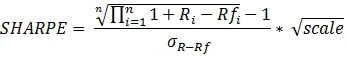
Use SHARPE to calculate the Sharpe ratio based upon return data. You have the option of computing the Sharpe ratio using either simple returns or geometric returns. For simple returns, the Sharpe ratio is calculated as the mean difference of the returns minus the risk-free rate divided by the standard deviation of the difference multiplied by the square root of a scale factor supplied to the function. For daily returns the scale factor might be 252; for weekly returns 52; for monthly returns 12. For the sake of consistency, the risk-free rate should be in the same units as the scaling factor.
For geometric returns, the Sharpe ratio is calculated as the geometric mean of the difference between the return and the risk free rate minus one, divided by the standard deviation of the difference multiplied by the square root of the scaling factor.
Syntax
Arguments
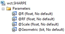
@R
the return value; the percentage return in floating point format (i.e. 10% = 0.10). @R is an expression of type float or of a type that can be implicitly converted to float.
@RF
the risk-free rate. @RF is an expression of type float or of a type that can be implicitly converted to float.
@Scale
the scaling factor used in the calculation. @Scale is an expression of type float or of a type that can be implicitly converted to float.
@Geometric
identifies whether or not to use geometric returns in the calculation. @Geometric is an expression of type bit or of a type that can be implicitly converted to bit.
Return Type
float
Remarks
· If @Geometric IS NULL then @Geometric is set equal to 'False'.
· If @RF IS NULL then @RF is set equal to 0.
· If @Scale IS NULL them @Scale is set to 1.
· For daily returns set @Scale = 252.
· For weekly returns set @Scale = 52.
· For monthly returns set @Scale = 12.
· For quarterly returns set @Scale = 4.
· To calculate the Sharpe ratio using price data or portfolio values, use the SHARPE2 aggregate function.
· @Geometric must be the same for all rows in the GROUP BY
· @Scale must the same for all rows in the GROUP BY.
Examples
In this example we have return data for IBM and we want to calculate the simple Sharpe ratio assuming an annual risk-free rate of 0.10%.
SELECT wct.SHARPE(r,.001/cast(252 as float),252,'False') as SHARPE
FROM (VALUES
('IBM','2012-12-18',0.0107),
('IBM','2012-12-17',0.0097),
('IBM','2012-12-14',-0.0012),
('IBM','2012-12-13',-0.005),
('IBM','2012-12-12',-0.0064),
('IBM','2012-12-11',0.0082),
('IBM','2012-12-10',0.0035),
('IBM','2012-12-07',0.0119),
('IBM','2012-12-06',0.0056),
('IBM','2012-12-05',-0.0037),
('IBM','2012-12-04',-0.0006),
('IBM','2012-12-03',-0.0031),
('IBM','2012-11-30',-0.0076),
('IBM','2012-11-29',-0.0023),
('IBM','2012-11-28',0.0039),
('IBM','2012-11-27',-0.0086),
('IBM','2012-11-26',-0.0032),
('IBM','2012-11-23',0.0168),
('IBM','2012-11-21',0.0058),
('IBM','2012-11-20',-0.006),
('IBM','2012-11-19',0.0182),
('IBM','2012-11-16',0.0059),
('IBM','2012-11-15',0.0018),
('IBM','2012-11-14',-0.0149),
('IBM','2012-11-13',-0.0049),
('IBM','2012-11-12',-0.0021),
('IBM','2012-11-09',-0.0024),
('IBM','2012-11-08',-0.0055),
('IBM','2012-11-07',-0.0158),
('IBM','2012-11-06',0.0048),
('IBM','2012-11-05',0.0036),
('IBM','2012-11-02',-0.0188),
('IBM','2012-11-01',0.0135)
)n(ticker,tdate,r)
This produces the following result.
SHARPE
----------------------
0.630146290350507
In this example, we have monthly returns for portfolio and monthly risk-free rates.
SELECT wct.SHARPE(r,rf,12,'False') as SHARPE
FROM (VALUES
('2011-01-31',0.009416,0.004986),
('2011-02-28',0.013579,0.005009),
('2011-03-31',0.009315,0.00495),
('2011-04-30',0.018145,0.005082),
('2011-05-31',0.007068,0.005112),
('2011-06-30',0.006657,0.005066),
('2011-07-31',0.006028,0.004967),
('2011-08-31',0.004719,0.005018),
('2011-09-30',0.018247,0.005011),
('2011-10-31',0.001731,0.004863),
('2011-11-30',0.002923,0.004825),
('2011-12-31',0.018072,0.004895),
('2012-01-31',0.0102,0.00507),
('2012-02-29',0.014619,0.005088),
('2012-03-31',0.017633,0.004956),
('2012-04-30',0.010065,0.005025),
('2012-05-31',0.012939,0.004736),
('2012-06-30',0.008044,0.004933),
('2012-07-31',0.017269,0.004969),
('2012-08-31',0.010842,0.004814),
('2012-09-30',0.009544,0.004959),
('2012-10-31',0.008508,0.005083),
('2012-11-30',0.000504,0.004977),
('2012-12-31',0.015876,0.004992),
('2013-01-31',0.00385,0.005003),
('2013-02-28',0.002251,0.004997),
('2013-03-31',0.013098,0.004815),
('2013-04-30',0.013069,0.005026),
('2013-05-31',0.006818,0.005013),
('2013-06-30',0.013184,0.005044),
('2013-07-31',0.013902,0.004822),
('2013-08-31',0.007957,0.005019),
('2013-09-30',0.003052,0.00487),
('2013-10-31',0.013372,0.005153),
('2013-11-30',0.014231,0.004994),
('2013-12-31',0.011182,0.004966)
)n(pdate,r,rf)
This produces the following result.
SHARPE
----------------------
3.58446805338759
In this example, we use weekly returns and calculate the Sharpe ratio using geometric returns.
SELECT wct.SHARPE(r,rf,52,'True') as SHARPE
FROM (VALUES
('IBM','2012-12-17',0.0173,0.000195),
('IBM','2012-12-10',-0.001,0.000194),
('IBM','2012-12-03',0.0099,0.000192),
('IBM','2012-11-26',-0.0177,0.000193),
('IBM','2012-11-19',0.035,0.00019),
('IBM','2012-11-12',-0.0142,0.000192),
('IBM','2012-11-05',-0.0153,0.000193),
('IBM','2012-10-31',0.0008,0.000192),
('IBM','2012-10-22',-0.0005,0.000192),
('IBM','2012-10-15',-0.0695,0.000193),
('IBM','2012-10-08',-0.0133,0.000193),
('IBM','2012-10-01',0.0151,0.00019),
('IBM','2012-09-24',0.0072,0.000189),
('IBM','2012-09-17',-0.004,0.000189),
('IBM','2012-09-10',0.0367,0.000199),
('IBM','2012-09-04',0.0239,0.000189),
('IBM','2012-08-27',-0.0148,0.000191),
('IBM','2012-08-20',-0.0171,0.000193),
('IBM','2012-08-13',0.0097,0.000192),
('IBM','2012-08-06',0.0082,0.000195),
('IBM','2012-07-30',0.0108,0.000192),
('IBM','2012-07-23',0.0204,0.000192),
('IBM','2012-07-16',0.0347,0.000192),
('IBM','2012-07-09',-0.0282,0.000194),
('IBM','2012-07-02',-0.0213,0.000192),
('IBM','2012-06-25',0.0097,0.00019),
('IBM','2012-06-18',-0.0271,0.00019),
('IBM','2012-06-11',0.0203,0.000194),
('IBM','2012-06-04',0.032,0.00019),
('IBM','2012-05-29',-0.0268,0.000192),
('IBM','2012-05-21',-0.0081,0.000192),
('IBM','2012-05-14',-0.0263,0.000195),
('IBM','2012-05-07',-0.0145,0.000196),
('IBM','2012-04-30',-0.0088,0.000191),
('IBM','2012-04-23',0.0361,0.000192),
('IBM','2012-04-16',-0.0158,0.000193),
('IBM','2012-04-09',-0.013,0.000196),
('IBM','2012-04-02',-0.0152,0.00019),
('IBM','2012-03-26',0.0154,0.000195),
('IBM','2012-03-19',-0.0026,0.000191),
('IBM','2012-03-12',0.0269,0.000188),
('IBM','2012-03-05',0.0091,0.000191),
('IBM','2012-02-27',0.0053,0.000191),
('IBM','2012-02-21',0.0224,0.000194),
('IBM','2012-02-13',0.0052,0.000193),
('IBM','2012-02-06',-0.0024,0.000194),
('IBM','2012-01-30',0.0167,0.000191),
('IBM','2012-01-23',0.0103,0.000193),
('IBM','2012-01-17',0.0523,0.000191),
('IBM','2012-01-09',-0.0185,0.000189)
)n(ticker,tdate,r, rf)
This produces the following result.
SHARPE
----------------------
0.478892083019103
In this example, we look at monthly returns for several different symbols and group the results by symbol. The risk-free rate is contained in the table with a ticker of 'LIB'
('IBM','2012-12-03',0.0264),
('IBM','2012-11-01',-0.0186),
('IBM','2012-10-01',-0.0623),
('IBM','2012-09-04',0.0647),
('IBM','2012-08-01',-0.0015),
('IBM','2012-07-02',0.0021),
('IBM','2012-06-01',0.0139),
('IBM','2012-05-01',-0.0646),
('IBM','2012-04-02',-0.0075),
('IBM','2012-03-01',0.0605),
('IBM','2012-02-01',0.0254),
('IBM','2012-01-03',0.0474),
('IBM','2011-12-01',-0.0219),
('MSFT','2012-12-03',0.0259),
('MSFT','2012-11-01',-0.0597),
('MSFT','2012-10-01',-0.041),
('MSFT','2012-09-04',-0.0343),
('MSFT','2012-08-01',0.0527),
('MSFT','2012-07-02',-0.0365),
('MSFT','2012-06-01',0.048),
('MSFT','2012-05-01',-0.0823),
('MSFT','2012-04-02',-0.0076),
('MSFT','2012-03-01',0.0164),
('MSFT','2012-02-01',0.0818),
('MSFT','2012-01-03',0.1374),
('MSFT','2011-12-01',0.0149),
('GOOG','2012-12-03',0.0311),
('GOOG','2012-11-01',0.0266),
('GOOG','2012-10-01',-0.0983),
('GOOG','2012-09-04',0.1013),
('GOOG','2012-08-01',0.0823),
('GOOG','2012-07-02',0.0912),
('GOOG','2012-06-01',-0.0014),
('GOOG','2012-05-01',-0.0397),
('GOOG','2012-04-02',-0.0567),
('GOOG','2012-03-01',0.0372),
('GOOG','2012-02-01',0.0657),
('GOOG','2012-01-03',-0.1019),
('GOOG','2011-12-01',0.0776),
('AAPL','2012-12-03',-0.1008),
('AAPL','2012-11-01',-0.0124),
('AAPL','2012-10-01',-0.1076),
('AAPL','2012-09-04',0.0028),
('AAPL','2012-08-01',0.0939),
('AAPL','2012-07-02',0.0458),
('AAPL','2012-06-01',0.0109),
('AAPL','2012-05-01',-0.0107),
('AAPL','2012-04-02',-0.026),
('AAPL','2012-03-01',0.1053),
('AAPL','2012-02-01',0.1883),
('AAPL','2012-01-03',0.1271),
('AAPL','2011-12-01',0.0597),
('ORCL','2012-12-03',0.0653),
('ORCL','2012-11-01',0.0353),
('ORCL','2012-10-01',-0.0099),
('ORCL','2012-09-04',-0.006),
('ORCL','2012-08-01',0.048),
('ORCL','2012-07-02',0.0187),
('ORCL','2012-06-01',0.122),
('ORCL','2012-05-01',-0.0996),
('ORCL','2012-04-02',0.0104),
('ORCL','2012-03-01',-0.0035),
('ORCL','2012-02-01',0.0373),
('ORCL','2012-01-03',0.102),
('ORCL','2011-12-01',-0.1818),
('LIB','2012-12-03',0.000834),
('LIB','2012-11-01',0.000831),
('LIB','2012-10-01',0.000842),
('LIB','2012-09-04',0.000839),
('LIB','2012-08-01',0.00084),
('LIB','2012-07-02',0.000834),
('LIB','2012-06-01',0.000832),
('LIB','2012-05-01',0.000841),
('LIB','2012-04-02',0.000839),
('LIB','2012-03-01',0.000835),
('LIB','2012-02-01',0.000822),
('LIB','2012-01-03',0.000831),
('LIB','2011-12-01',0.000829)
)n(ticker,tdate,r)
SELECT s1.ticker
,wct.SHARPE(s1.r,s2.r,12,'True') as SHARPE
FROM #s s1
JOIN #s s2
ON s1.tdate = s2.tdate
WHERE s2.ticker = 'LIB'
AND s1.ticker <> 'LIB'
GROUP BY s1.ticker
DROP TABLE #s
This produces the following result.
ticker SHARPE
------ ----------------------
AAPL 0.995989470993115
GOOG 0.654852585110675
IBM 0.278777751558357
MSFT 0.358326233029484
ORCL 0.29019079070248
See Also