LOGIT
Updated: 27 February 2015
Use the table-valued function LOGIT to calculate the binary logistic regression coefficients from a table of x-values (the independent variables) and dichotomous y-values (the dependent variable). The function supports the entry of the data in raw form, where the y-values are a column of zeros and ones {0,1}. The y-value can appear in any column and the column number of the y-values is specified at input.
|
x1
|
x2
|
x3
|
…
|
xn
|
y
|
|
x1,1
|
x1,2
|
x1,3
|
…
|
x1,n
|
y1
|
|
x2,1
|
x2,2
|
x2,3
|
…
|
x2,n
|
y2
|
|
…
|
…
|
…
|
…
|
…
|
…
|
|
xm,1
|
xm,2
|
xm,3
|
…
|
xm,n
|
ym
|
For summary values, where the y-values are the counts of successes and failures, use the LOGITSUM function.
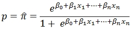
Logistic regression estimates the probability of an event occurring. Unlike ordinary least squares (see LINEST and LINEST_q) which estimates the value of a dependent variable based on the independent variables, LOGIT measures the probability (p) of an event occurring (1) or not occurring (0). The probability is estimated as:
The LOGIT function works by finding the coefficient (ß) values that maximize the log-likelihood statistic, which is defined as:
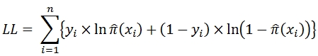
using a method of iteratively re-weighted least squares.
Syntax
SELECT * FROM [wct].[LOGIT](
<@Matrix_RangeQuery, nvarchar(max),>
,<@y_ColumnNumber, int,>)
@Matrix_RangeQuery
the SELECT statement, as a string, which, when executed, creates the resultant table of x- and y-values used in the calculation.
@y_ColumnNumber
the number of the column in the resultant table returned by @Matrix_RangeQuery which contains the dichotomous outcomes. @y_ColumnNumber must be of the type int or of a type that implicitly converts to int.
Return Types
RETURNS TABLE(
[stat_name] [nvarchar](10) NULL,
[idx] [int] NULL,
[stat_val] [float] NULL
)
Table Description
stat_name
Identifies the statistic being returned:
|
b
|
estimated coefficient for each independent variable plus the intercept
|
|
se
|
standard error of b
|
|
z
|
z statistic for b
|
|
pval
|
p-value (normal distribution) for the z statistic
|
|
Wald
|
Wald statistic
|
|
LL0
|
log-likelihood with just the intercept and no other coefficients
|
|
LLM
|
model log-likelihood
|
|
chisq
|
chi squared statistic
|
|
df
|
degrees of freedom
|
|
p_chisq
|
p-value of the chi-squared statistic
|
|
AIC
|
Akaike information criterion
|
|
BIC
|
Bayesian information criterion
|
|
Nobs
|
number of observations
|
|
rsql
|
log-linear ratio R2
|
|
rsqcs
|
Cox and Snell's R2
|
|
rsqn
|
Nagelkerke's R2
|
|
D
|
deviance
|
|
Iterations
|
number of iteration in iteratively re-weighted least squares
|
|
Converged
|
a bit value identifying whether a solution was found (1) or not (0)
|
|
AUROC
|
area under the ROC curve
|
For more information on how these statistics are calculated see the Examples.
idx
Identifies the subscript for the estimated coefficient (b), standard error of the coefficient (se),
z statistics (z), p-value of the z statistic (pval), and the Wald statistic.
When the idx is 0, it is referring to the intercept, otherwise the idx identifies the column number of independent variable.
Descriptive statistics other than the ones mentioned above will have an idx of NULL.
stat_val
the calculated value of the statistic.
Remarks
· If @y_ColumnNumber is NULL then the right-most column in the resultant table is assumed to contain the dichotomous results.
· @Matrix_RangeQuery must return at least 2 columns or an error will be returned.
· If @y_ColumnNumber is not NULL and @y_ColumnNumber < 1 an error will be returned.
· If @y_ColumnNumber is not NULL and @y_ColumnNumber greater than the number of columns returned by @Matrix_RangeQuery an error will be returned.
Examples
Example #1
In this example we use the Coronary Heart Disease data from Applied Logistic Regression, Third Edition by David W. Hosmer, Jr., Stanley Lemeshow, and Rodney X. Sturdivant. The data consist of a single independent variable (age) and an outcome (chd) which indicates the absence (0) or presence (1) of coronary heart disease.
The following SQL populates a temporary table, #chd.
SELECT
*
INTO
#chd
FROM (VALUES
(20,0),(23,0),(24,0),(25,0),(25,1),(26,0),(26,0),(28,0),(28,0),(29,0)
,(30,0),(30,0),(30,0),(30,0),(30,0),(30,1),(32,0),(32,0),(33,0),(33,0)
,(34,0),(34,0),(34,1),(34,0),(34,0),(35,0),(35,0),(36,0),(36,1),(36,0)
,(37,0),(37,1),(37,0),(38,0),(38,0),(39,0),(39,1),(40,0),(40,1),(41,0)
,(41,0),(42,0),(42,0),(42,0),(42,1),(43,0),(43,0),(43,1),(44,0),(44,0)
,(44,1),(44,1),(45,0),(45,1),(46,0),(46,1),(47,0),(47,0),(47,1),(48,0)
,(48,1),(48,1),(49,0),(49,0),(49,1),(50,0),(50,1),(51,0),(52,0),(52,1)
,(53,1),(53,1),(54,1),(55,0),(55,1),(55,1),(56,1),(56,1),(56,1),(57,0)
,(57,0),(57,1),(57,1),(57,1),(57,1),(58,0),(58,1),(58,1),(59,1),(59,1)
,(60,0),(60,1),(61,1),(62,1),(62,1),(63,1),(64,0),(64,1),(65,1),(69,1)
)n(age,chd)
We can run the following SQL to reproduce Table 1.2, Frequency Table of Age Group by CHD from the Hosmer book, verifying that we are using the same data.
SELECT
a.descr as [Age Group]
,COUNT(*) as n
,COUNT(*) - SUM(c.chd) as Absent
,SUM(c.chd) as Present
,AVG(cast(c.chd as float)) as Mean
FROM
#chd c
CROSS APPLY(
SELECT TOP 1
grp
,descr
FROM (VALUES
(20,1,'20-29'),(30,2,'30-34'),(35,3,'35-39'),(40,4,'40-44')
,(45,5,'45-49'),(50,6,'50-55'),(55,7,'55-59'),(60,8,'60-69')
)n(age,grp,descr)
WHERE
n.age <= c.age
ORDER BY
n.age DESC
)a
GROUP BY
a.descr
,a.grp
ORDER BY
1
This produces the following result.
This SQL calculates the results of the logistic regression.
SELECT
*
FROM
wct.LOGIT(
'SELECT
age
,chd
FROM
#chd'
,2
)
This produces the following result.
Let's reformat some of these to make them easier to read and easier to compare to Hosmer. This SQL reproduces Table 1.3, Results of Fitting the Logistic Regression to the CHDAGE Data, n = 100.
SELECT
n.Variable
,p.b as Coeff
,p.se as [Std. Err]
,p.z
,p.pval as p
FROM (
SELECT
*
FROM
wct.LOGIT(
'SELECT
age
,chd
FROM
#chd'
,2
)
)d
PIVOT(
SUM(stat_val)
FOR
stat_name
IN
(b,se,z,pval)
)p
CROSS APPLY(
VALUES (0,'Constant'),(1,'Age')
)n(idx,variable)
WHERE
p.idx = n.idx
ORDER BY
p.idx DESC
This produces the following result.
As Hosmer points out, the fitted values, are given by the equation
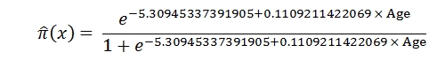
meaning that we can use this equation to predict the probability of the presence of coronary heart disease given a person's age.
If you are not interested in an explanation of how the remaining statistics are calculated, then skip to the next example. In order to explore how these remaining statistics are calculated, let's store the results of the LOGIT function in a table (#mylogit) with the following SQL.
SELECT
stat_name
,idx
,stat_val
INTO
#mylogit
FROM
wct.LOGIT(
'SELECT
age
,chd
FROM
#chd'
,2
)
The standard errors of the coefficients (se) can be calculated as the square root of the diagonal of the covariance matrix:

Where X is the design matrix (a column of ones added to the input data) and W is the diagonal matrix of weights calculated by the iteratively re-weighted least squares process.
In this piece of SQL we will create a table which calculates the log-likelihood (LL), the weights (W) and the predicted value, which can then be used to calculate the covariance matrix.
SELECT
*
,(p_obs*LOG(p_pred)+(1-p_obs)*LOG(1-p_pred)) as LL
,p_pred*(1-p_pred) as W
INTO
#m
FROM (
SELECT
age
,chd as p_obs
,EXP(b0.stat_val + age * b1.stat_val)/(1+EXP(b0.stat_val + age * b1.stat_val)) as p_pred
FROM
#mylogit b0
JOIN
#mylogit b1
ON
b0.stat_name = 'b'
AND b0.idx = 0
AND b1.stat_name = 'b'
AND b1.idx = 1
CROSS JOIN
#chd
)n
We can now use the matrix functions from the XLeratorDB math module to verify the results returned by the LOGIT function for the standard errors (se).
SELECT
RowNum as idx
,SQRT(ItemValue) as se
FROM
wct.Matrix(
wct.MATINVERSE(
wct.MATMULT(
wct.TRANSPOSE(
wct.Matrix2String_q('SELECT 1, age FROM #m')
)
,wct.Matrix2String_q('SELECT W, W * age FROM #m')
)
)
)
WHERE
RowNum = ColNum
DROP TABLE
#chd
This produces the following result.
From the coefficients (b) and the se values, we can calculate the z, pval, and Wald values. The following SQL demonstrates the calculation, using the b and se values stored in #mylogit.
SELECT
n.Variable
,p.b / p.se as z
,2 * wct.NORMSDIST(-ABS(p.b / p.se)) as pval
,POWER(p.b / p.se, 2) as Wald
FROM (
SELECT
*
FROM
#mylogit
)d
PIVOT(
SUM(stat_val)
FOR
stat_name
IN
(b,se)
)p
CROSS APPLY(
VALUES (0,'Constant'),(1,'Age')
)n(idx,variable)
WHERE
p.idx = n.idx
ORDER BY
p.idx DESC
This produces the following result.
The model log-likelihood (LLM) is simply the sum of the individual log-likelihoods which we have already computed and stored in #m.
SELECT
SUM(LL) as LLM
FROM
#m
This produces the following result.
The calculation of LL0 can be done directly from the input data.
SELECT
f*LOG(f) + s*LOG(s) - n*LOG(n) as LL0
FROM (
SELECT
COUNT(*) as n
,SUM(chd) as s
,COUNT(*) - SUM(chd) as f
FROM
#chd
)n
This produces the following result
Given LL0 and LLM it is relatively straightforward to calculate the rest of the statistics.
SELECT
x.*
FROM (
SELECT
2 *(LLM - LL0) as chisq
,wct.CHIDIST(2 *(LLM - LL0), df) as pchisq
,-2 *(LLM - df - 1) as AIC
,-2 * LLM + LOG(Nobs) *(df + 1) as BIC
,1 - LLM/LL0 as rsql
,1 - EXP((-2/Nobs)*(LLM-LL0)) as rsqcs
,(1 - EXP((-2/Nobs)*(LLM-LL0)))/(1-exp(2*LL0/Nobs)) as rsqn
,-2*LOG(LL0/LLM) as D
FROM (
SELECT
stat_name
,stat_val
FROM
#mylogit
)d
PIVOT(
SUM(stat_val)
FOR
stat_name
IN
(LL0,LLM,df,Nobs)
)p
)q
CROSS APPLY(
VALUES
('chisq',chisq),
('pchisq',pchisq),
('AIC',AIC),
('BIC',BIC),
('rsql',rsql),
('rsqcs',rsqcs),
('rsqn',rsqn),
('D',D)
)x(stat_name, stat_val)
This produces the following result.
We can use the table-valued function ROCTable for the calculation of the area under the ROC curve (AUROC). The table-valued function requires the predicted probabilities and associated absence (0) or presence (1) of coronary heart disease as inputs. We will use the LOGITPRED function to create these combinations and store them in a temporary table which will then be called from ROCTable.
SELECT
wct.LOGITPRED('SELECT stat_val FROM #mylogit where stat_name = ''b'' ORDER BY idx',cast(age as varchar(max))) as [p predicted]
,chd as y
INTO
#t
FROM
#chd
SELECT
*
FROM
wct.ROCTABLE('SELECT * FROM #t')
This produces the following result.
You can get more information about the calculation of the area under the ROC curve by going to the ROCTable documentation
Example #2
The dataset contains 4 columns of data which are labeled admit, gre, gpa, and rank. The variables gpa and gre will be treated as continuous. The variable rank has the values 1 through 4 where a 1 indicates the highest-ranked institutions and a 4 indicates the lowest-ranked institutions.
We can run the following SQL to get some basic descriptive statistics to make sure that the data are loaded correctly.
SELECT
n.lbl,
wct.QUARTILE(admit,n.x) as Admit,
wct.QUARTILE(gre,n.x) as gre,
wct.QUARTILE(gpa,n.x) as gpa,
wct.QUARTILE(rank,n.x) as rank
FROM
#mydata
CROSS APPLY(VALUES
('Min',0),('1st Quartile',1),('Median',2),('3rd Quartile',3),('Max',4))n(lbl,x)
GROUP BY
n.lbl
UNION
SELECT
'Mean',
AVG(cast(admit as float)) as Admit,
AVG(cast(gre as float)) as gre,
AVG(cast(gpa as float)) as gpa,
AVG(cast(rank as float)) as rank
FROM
#mydata
ORDER BY
3
This produces the following result.
To get the standard deviations, we could run the following SQL.
SELECT
wct.STDEV_S(admit) as Admit,
wct.STDEV_S(gre) as gre,
wct.STDEV_S(gpa) as gpa,
wct.STDEV_S(rank) as rank
FROM
#mydata
This produces the following result.
This SQL will create a two-way contingency table between the admit outcome and the rank predictor. We run this SQL to check to see if there are any zeroes in the contingency table.
SELECT
admit,[1],[2],[3],[4]
FROM (
SELECT admit, rank FROM #mydata
) p
PIVOT(
COUNT([rank]) FOR [rank] IN([1],[2],[3],[4])
) as d
This produces the following result.
This SQL will run the logistic regression and put the results in a temporary table, #mylogit. The only reason for storing the results in the temp table is to make it easier to follow the rest of the example.
SELECT
*
INTO
#mylogit
FROM
wct.LOGIT(
'SELECT
admit
,gre
,gpa
,CASE RANK
WHEN 2 THEN 1
ELSE 0
END
,CASE RANK
WHEN 3 THEN 1
ELSE 0
END
,CASE RANK
WHEN 4 THEN 1
ELSE 0
END
FROM
#mydata'
,1
)
Note that we have taken the rank column and turned it into 3 columns, representing the ranks of 2, 3, and 4, since we are treating the rank variable as discrete and not continuous.
In this SQL, we are going to select the estimated coefficients, the standard error of the estimates, the z-value, and the probability associated with that z-value, and return the results in spreadsheet format with the appropriate labels for the estimated coefficients.
SELECT
CASE idx
WHEN 0 THEN 'Intercept'
WHEN 1 THEN 'gre'
WHEN 2 THEN 'gpa'
WHEN 3 THEN 'rank2'
WHEN 4 THEN 'rank3'
WHEN 5 THEN 'rank4'
END as [X]
,ROUND(b,5) as [Estimated]
,ROUND(se,5) as [Std. Error]
,ROUND(z,2) as [z Value]
,ROUND(pval,5) as [Pr(>|z|)]
,ROUND(Wald,2) as Wald
FROM
#mylogit
PIVOT(
SUM(stat_val) FOR stat_name IN(b,se,z,pval,Wald)
) as pvt
WHERE
idx IS NOT NULL
ORDER BY
idx
This produces the following result.
The results of the regression indicate that both the gre and gpa are statistically significant as are the three terms for rank. You could interpret the results in the following way:
o for every one unit change in gre, the log odds of success (admission) increase by 0.00226.
o for every one unit change in gpa, the log odds of success increase by 0.80404.
o since the rank variable is not continuous it is interpreted differently. For example, attending an undergraduate institution with a rank of 2 (as opposed to 1) decreases the log odds of admission by 0.67544.
The following SQL returns the remaining statistics from the regression analysis.
SELECT
stat_name
,stat_val
FROM
#mylogit
WHERE
idx IS NULL
This produces the following result.
See Also