New SQL Server Interpolation Functions in XLeratorDB
Apr
20
Written by:
Charles Flock
4/20/2011 5:02 PM

A look at the new interpolation functions in XLeratorDB/math2008 written specifically for SQL Server 2008.
We are happy to announce the latest release of XLeratorDB/math and the initial release of XLeratorDB/math2008, specifically written for SQL Server 2008.
XLeratorDB/math2008 contains multi-input aggregate functions to do the following types of interpolations:
· Linear
· Cubic Spline
· Polynomial
It also contains a curve-fitting function, letting you specify the degree of the polynomial that you would like to fit to the x- and y-values supplied to the function.
Let’s look at these functions by creating some x- and y-values and then using them to calculate a new y-value for a supplied new x-value. In this example, we will create x- and y-values based on the sine function.
SELECT x
,SIN(x) as y
FROM (VALUES
(0)
,(PI()/4)
,(2*PI()/4)
,(3*PI()/4)
,(4*PI()/4)
,(5*PI()/4)
,(6*PI()/4)
,(7*PI()/4)
,(8*PI()/4)
) n(x)
This produces the following result.
x y
---------------------- ----------------------
0 0
0.785398163397448 0.707106781186547
1.5707963267949 1
2.35619449019234 0.707106781186548
3.14159265358979 1.22464679914735E-16
3.92699081698724 -0.707106781186547
4.71238898038469 -1
5.49778714378214 -0.707106781186548
6.28318530717959 -2.44929359829471E-16
Let’s find the interpolated value at x = 2.0 using linear interpolation on the derived table. We would simply enter the following SQL.
SELECT 2.0 as new_x
,wct.INTERP(x, y, 2.0) as LINEAR
FROM (
SELECT x
,SIN(x) as y
FROM (VALUES
(0)
,(PI()/4)
,(2*PI()/4)
,(3*PI()/4)
,(4*PI()/4)
,(5*PI()/4)
,(6*PI()/4)
,(7*PI()/4)
,(8*PI()/4)
) n(x)
) m(x,y)
This produces the following result.
new_x LINEAR
----- ----------------------
2.0 0.839939980470792
This result is the linearly interpolated value of x, sometimes called straight-line interpolation, and was calculated using the function INTERP. The INTERP function is a multi-input aggregate function which takes as input a set of x- and y-values and a single new x-value. Straight-line interpolation, as its name implies, calculates the y-value of the new x-value by figuring out the slope of the line between the 2 x-values enveloping the new x-value. It is only ever concerned about 2 points. Because of this, straight-line interpolation is bound by the x-values. The new x-value must be between the minimum and maximum values of x in the set of x-values passed into the function.
Cubic spline interpolation, however, takes into consideration the ‘shape’ of the set of values passed into the function. This simply means that the calculation of a y-value given a new x-value, considers all the x- and y-values rather than just the surrounding x- and y-values. Because of this, the function is not bound by the limits of x, so it is possible to extrapolate as well as interpolate.
In the example, we have simply added spline interpolation to the SELECT statement, allowing us to compare the results of linear and spline interpolation as x = 2.
SELECT 2.0 as new_x
,wct.INTERP(x, y, 2.0) as LINEAR
,wct.SPLINE(x, y, 2.0) as SPLINE
FROM (
SELECT x
,SIN(x) as y
FROM (VALUES
(0)
,(PI()/4)
,(2*PI()/4)
,(3*PI()/4)
,(4*PI()/4)
,(5*PI()/4)
,(6*PI()/4)
,(7*PI()/4)
,(8*PI()/4)
) n(x)
) m(x,y)
This produces the following result.
new_x LINEAR SPLINE
----- ---------------------- ----------------------
2.0 0.839939980470792 0.908238566556583
Like the SPLINE function, POLYINTERP takes into consideration the ‘shape’ of the x-value and the y-values. POLYINTERP is an implementation of Neville’s algorithm, and constructs an approximating polynomial where the degree of the polynomial is one less than the number of rows in the set of x- and y-values supplied to the function. Like SPLINE, POLYINTERP is not bound by the minimum and maximum values of x, so it is possible to extrapolate as well as interpolate. We can simply add POLYINTERP to our example and compare the results.SELECT 2.0 as new_x
,wct.INTERP(x, y, 2.0) as LINEAR
,wct.SPLINE(x, y, 2.0) as LINEAR
,wct.POLYINTERP(x, y, 2.0) as POLYINTERP
FROM (
SELECT x
,SIN(x) as y
FROM (VALUES
(0)
,(PI()/4)
,(2*PI()/4)
,(3*PI()/4)
,(4*PI()/4)
,(5*PI()/4)
,(6*PI()/4)
,(7*PI()/4)
,(8*PI()/4)
) n(x)
) m(x,y)
This produces the following result.
new_x LINEAR SPLINE POLYINTERP
----- ---------------------- ---------------------- ----------------------
2.0 0.839939980470792 0.908238566556583 0.909373773636468
It’s quite plain to see that each of the interpolation techniques produced a different answer. It’s important to remember that interpolation, by definition, only supplies an approximate answer. In this example, we are approximating a function (the sine function), so it is quite easy to evaluate the goodness of fit by comparing the interpolated value to the value of the function at the new x-value.
SELECT 2.0 as new_x
,ROUND(wct.INTERP(x, y, 2.0), 8) as LINEAR
,ROUND(wct.SPLINE(x, y, 2.0), 8) as SPLINE
,ROUND(wct.POLYINTERP(x, y, 2.0), 8) as POLYINTERP
,ROUND(SIN(2.0), 8) as [FUNCTION]
FROM (
SELECT x
,SIN(x) as y
FROM (VALUES
(0)
,(PI()/4)
,(2*PI()/4)
,(3*PI()/4)
,(4*PI()/4)
,(5*PI()/4)
,(6*PI()/4)
,(7*PI()/4)
,(8*PI()/4)
) n(x)
) m(x,y)
This produces the following result.
new_x LINEAR SPLINE POLYINTERP FUNCTION
----- ------------- ------------- ------------- -------------
2.0 0.83993998 0.90823857 0.90937377 0.90929743
It looks like POLYINTERP produces the best approximation of the sine function at x = 2.
In this example, we will put the x- and y-values into a temporary table and then use the XLeratorDB SERIESFLOAT function to generate new x-values in increments of 0.25 in the range [0, 6] and calculate the interpolated values.
SELECT x
,SIN(x) as y
into #xy
FROM (VALUES
(0)
,(PI()/4)
,(2*PI()/4)
,(3*PI()/4)
,(4*PI()/4)
,(5*PI()/4)
,(6*PI()/4)
,(7*PI()/4)
,(8*PI()/4)
) n(x)
SELECT k.SeriesValue as new_x
,ROUND(wct.INTERP(x, y, k.SeriesValue), 8) as LINEAR
,ROUND(wct.SPLINE(x, y, k.SeriesValue), 8) as SPLINE
,ROUND(wct.POLYINTERP(x, y, k.SeriesValue), 8) as POLYINTERP
,ROUND(SIN(k.SeriesValue), 8) as [FUNCTION]
FROM #xy, wct.SeriesFloat(0,6,0.25,NULL,NULL) k
GROUP BY k.SeriesValue, SIN(Seriesvalue)
ORDER BY 1
DROP TABLE #xy
This produces the following result.
new_x LINEAR SPLINE POLYINTERP FUNCTION
----- ------------- ------------- ------------- -------------
0 0 0 0 0
0.25 0.22507908 0.24696393 0.24860779 0.24740396
0.5 0.45015816 0.47912347 0.48010706 0.47942554
0.75 0.67523724 0.68167422 0.68169982 0.68163876
1 0.78713679 0.84072604 0.84126618 0.84147098
1.25 0.88036760 0.94800868 0.94881075 0.94898462
1.5 0.97359841 0.99738587 0.99745890 0.99749499
1.75 0.93317079 0.98347828 0.98404986 0.98398595
2 0.83993998 0.90823857 0.90937377 0.90929743
2.25 0.74670917 0.77775249 0.77809969 0.77807320
2.5 0.57763633 0.59842733 0.59844163 0.59847214
2.75 0.35255726 0.38121940 0.38160977 0.38166099
3 0.12747818 0.14082230 0.14109378 0.14112001
3.25 -0.09760090 -0.10795957 -0.10817465 -0.10819513
3.5 -0.32267998 -0.35032182 -0.35073293 -0.35078323
3.75 -0.54775906 -0.57146006 -0.57152537 -0.57156132
4 -0.73433360 -0.75660590 -0.75682062 -0.75680250
4.25 -0.82756441 -0.89396442 -0.89506157 -0.89498936
4.5 -0.92079522 -0.97689057 -0.97760076 -0.97753012
4.75 -0.98597398 -0.99925913 -0.99927420 -0.99929279
5 -0.89274317 -0.95802941 -0.95876657 -0.95892427
5.25 -0.79951236 -0.85808024 -0.85872061 -0.85893449
5.5 -0.70511451 -0.70554379 -0.70554391 -0.70554033
5.75 -0.48003543 -0.50803635 -0.50886570 -0.50827908
6 -0.25495635 -0.27895497 -0.28059686 -0.27941550
We can take this data and drop it into EXCEL and produce the following graph of the results.
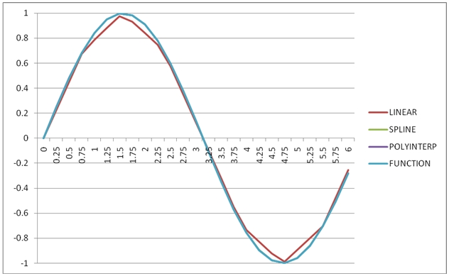
The graph plainly shows that SPLINE and POLYINTERP both produce results that are very similar to the function, while INTERP produces the least accurate results.
In this SQL we have substituted the ATAN function for the SIN function.
SELECT x
,ATAN(x) as y
into #xy
FROM (VALUES
(0)
,(PI()/4)
,(2*PI()/4)
,(3*PI()/4)
,(4*PI()/4)
,(5*PI()/4)
,(6*PI()/4)
,(7*PI()/4)
,(8*PI()/4)
) n(x)
SELECT k.SeriesValue as new_x
,ROUND(wct.INTERP(x, y, k.SeriesValue), 8) as LINEAR
,ROUND(wct.SPLINE(x, y, k.SeriesValue), 8) as SPLINE
,ROUND(wct.POLYINTERP(x, y, k.SeriesValue), 8) as POLYINTERP
,ROUND(ATAN(k.SeriesValue), 8) as [FUNCTION]
FROM #xy, wct.SeriesFloat(0,6,0.25,NULL,NULL) k
GROUP BY k.SeriesValue, SIN(Seriesvalue)
ORDER BY 1
DROP TABLE #xy
We can drop the resultant table into EXCEL and graph the results.
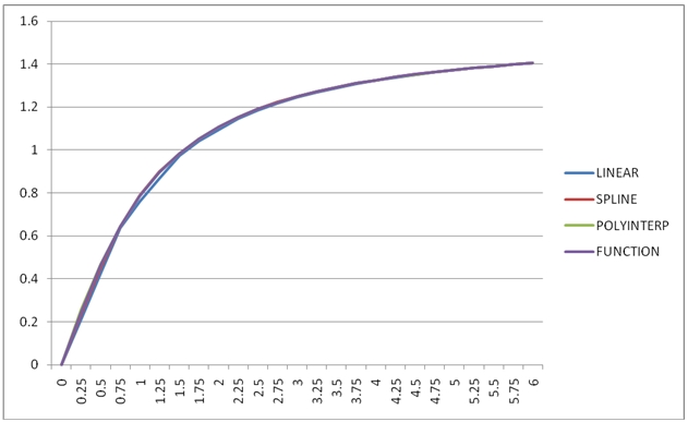
In this case, the LINEAR interpolation results are nearly as good as SPLINE and POLYINTERP.
So, which one should you use? That’s entirely up to you, of course, but now you can make that decision based solely on your business requirements rather than on the complexity of implementing interpolation on your own, since SQL Server has no native interpolation capabilities. With XLeratorDB/math2008 you can interpolate in a variety of ways, and on massive amounts of data, easily and efficiently. Try the 15-day free trial today.