Calculating a time-weighted rate of return using modified Dietz in SQL Server
Oct
24
Written by:
Charles Flock
10/24/2012 1:24 PM

The modified Dietz calculation produces a result which measures the performance of an investment portfolio based on time-weighted cash flows. Today, we will look at two XLeratorDB aggregate functions, EMDIETZ and FVSCHEDULE, which calculate the modified Dietz value for each period and then link the results together to come up with a time-weighted rate of return value.
The EMDIETZ aggregate function calculates the modified Dietz value for a given period. We were recently asked by one of our customers if there was some easy way to link the EMDIETZ results together so that the linked results could be used as a time-weighted rate of return calculation. In other words, was there some easy way to perform this calculation?
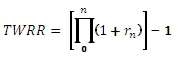
Where rn is the modified Dietz result for each period.
The FVSCHEDULE function lets us do this quite easily and today we are going to look at some simple SQL that will automatically calculate the modified Dietz values within a quarter and then link those results together to return a time-weighted rate of return value for the quarter.
Let’s say you had the following data, and you want to use the modified Dietz to calculate a time-weighted rate of return for the quarter.
date_tran amt_tran descr_tran
----------- --------------------- ----------
28 Jun 2012 498987.32 MV
05 Jul 2012 -993.58 Withdrawal
10 Jul 2012 1000.30 Deposit
16 Jul 2012 -954.15 Withdrawal
20 Jul 2012 839.55 Deposit
25 Jul 2012 36124.27 Deposit
25 Jul 2012 493997.45 MV
31 Jul 2012 503977.19 MV
03 Aug 2012 -930.18 Withdrawal
09 Aug 2012 828.23 Deposit
14 Aug 2012 -938.37 Withdrawal
20 Aug 2012 1090.90 Deposit
24 Aug 2012 -48246.35 Withdrawal
24 Aug 2012 498937.42 MV
29 Aug 2012 509016.96 MV
04 Sep 2012 -922.09 Withdrawal
07 Sep 2012 1090.67 Deposit
13 Sep 2012 -916.77 Withdrawal
18 Sep 2012 1044.57 Deposit
24 Sep 2012 35643.60 Deposit
24 Sep 2012 503926.79 MV
28 Sep 2012 514107.13 MV
Our input consists of a transaction date (date_tran), a transaction amount (amt_tran), and a transaction description (descr_tran). For purposes of this example, there are only three transaction descriptions: Deposit, Withdrawal, and MV (market value). Market values are supplied on the last business day of a month and on any date on which there has been a significant change in the account. The market value is always greater than zero and the ending market value for one period becomes the beginning market value for the next period.
Let’s put this data into a table.
CREATE TABLE #m(
date_tran date,
amt_tran money,
descr_tran nvarchar(10)
)
INSERT INTO #m VALUES ('2012-06-28',498987.32,'MV')
INSERT INTO #m VALUES ('2012-07-05',-993.58,'Withdrawal')
INSERT INTO #m VALUES ('2012-07-10',1000.3,'Deposit')
INSERT INTO #m VALUES ('2012-07-16',-954.15,'Withdrawal')
INSERT INTO #m VALUES ('2012-07-20',839.55,'Deposit')
INSERT INTO #m VALUES ('2012-07-25',36124.27,'Deposit')
INSERT INTO #m VALUES ('2012-07-25',493997.45,'MV')
INSERT INTO #m VALUES ('2012-07-31',503977.19,'MV')
INSERT INTO #m VALUES ('2012-08-03',-930.18,'Withdrawal')
INSERT INTO #m VALUES ('2012-08-09',828.23,'Deposit')
INSERT INTO #m VALUES ('2012-08-14',-938.37,'Withdrawal')
INSERT INTO #m VALUES ('2012-08-20',1090.9,'Deposit')
INSERT INTO #m VALUES ('2012-08-24',-48246.35,'Withdrawal')
INSERT INTO #m VALUES ('2012-08-24',498937.42,'MV')
INSERT INTO #m VALUES ('2012-08-29',509016.96,'MV')
INSERT INTO #m VALUES ('2012-09-04',-922.09,'Withdrawal')
INSERT INTO #m VALUES ('2012-09-07',1090.67,'Deposit')
INSERT INTO #m VALUES ('2012-09-13',-916.77,'Withdrawal')
INSERT INTO #m VALUES ('2012-09-18',1044.57,'Deposit')
INSERT INTO #m VALUES ('2012-09-24',35643.6,'Deposit')
INSERT INTO #m VALUES ('2012-09-24',503926.79,'MV')
INSERT INTO #m VALUES ('2012-09-28',514107.13,'MV')
The EMDIETZ function is designed to calculate the return for a single period. In this example, the periods are identified as those dates having a transaction description of 'MV'. In this example, the periods are contiguous so that the end date of one period becomes the start date for the next period. This makes the calculation of the start and end dates relatively straightforward. The following SQL will calculate the start and end dates and put the results into a temporary table, #d.
SELECT m1.date_tran as date_start
,MIN(m2.date_tran) as date_end
INTO #d
FROM #m m1
JOIN #m m2
ON m1.descr_tran = 'MV'
AND m2.descr_tran = 'MV'
AND m2.date_tran > m1.date_tran
GROUP BY m1.date_tran
Here are the contents of the table (#d).
date_start date_end
---------- ----------
2012-06-28 2012-07-25
2012-07-25 2012-07-31
2012-07-31 2012-08-24
2012-08-24 2012-08-29
2012-08-29 2012-09-24
2012-09-24 2012-09-28
Knowing the start and the end dates, we can write a SELECT statement which will calculate the modified Dietz value for each of the above periods. The EMDIETZ function expects the ending market value for a period to be negative and the starting market value for the period to be positive.
Since EMDIETZ is an aggregate function, it is very simple to group the cash flows and the modified Dietz calculation into the appropriate periods. We can manipulate the beginning and ending market values simply by using a CASE statement.
SELECT date_start
,date_end
,wct.EMDIETZ(
CASE
--Flip the sign for the ending market value
WHEN descr_tran = 'MV' and date_tran = date_end THEN -amt_tran
--Don't include prior period transactions
WHEN descr_tran <> 'MV' and date_tran = date_start THEN 0
ELSE amt_tran
END,
date_tran) as [Dietz]
FROM #d
JOIN #m
ON #m.date_tran BETWEEN #d.date_start and #d.date_end
GROUP BY date_start, date_end
This produces the following result.
date_start date_end Dietz
---------- ---------- ----------------------
2012-06-28 2012-07-25 -0.0822354637534845
2012-07-25 2012-07-31 0.0202020071156238
2012-07-31 2012-08-24 0.085716824301861
2012-08-24 2012-08-29 0.0202020125089035
2012-08-29 2012-09-24 -0.0806292943843924
2012-09-24 2012-09-28 0.0202020218055881
To calculate the time-weighted rate of return for the quarter, we can simply link the Dietz values together using the FVSCHEDULE function.
SELECT wct.FVSCHEDULE(Dietz) - 1 as TWRR
FROM (
SELECT date_start
,date_end
,wct.EMDIETZ(
CASE
--Flip the sign for the ending market value
WHEN descr_tran = 'MV' and date_tran = date_end THEN -amt_tran
--Don't include prior period transactions
WHEN descr_tran <> 'MV' and date_tran = date_start THEN 0
ELSE amt_tran
END,
date_tran) as [Dietz]
FROM #d
JOIN #m
ON #m.date_tran BETWEEN #d.date_start and #d.date_end
GROUP BY date_start, date_end
) n
This produces the following result.
TWRR
----------------------
-0.0272594273584182
Now that we have the basic principles down, let’s look at how we can adapt this query so that we can perform this calculation for multiple accounts. We will set up some test data and the accounts will have differing transactions and market values, but there will always be a market value for the last business day of the month or the date that the account is closed. We start by creating a new temporary table which has an additional column, id_acct, which is an account identifier.
CREATE TABLE #m2(
id_acct nchar(4),
date_tran date,
amt_tran money,
descr_tran nvarchar(10)
)
We populate this table with some data.
INSERT INTO #m2 VALUES ('msta','2012-06-28',498987.32,'MV')
INSERT INTO #m2 VALUES ('msta','2012-07-05',-993.58,'Withdrawal')
INSERT INTO #m2 VALUES ('msta','2012-07-10',1000.3,'Deposit')
INSERT INTO #m2 VALUES ('msta','2012-07-16',-954.15,'Withdrawal')
INSERT INTO #m2 VALUES ('msta','2012-07-20',839.55,'Deposit')
INSERT INTO #m2 VALUES ('msta','2012-07-25',36124.27,'Deposit')
INSERT INTO #m2 VALUES ('msta','2012-07-25',493997.45,'MV')
INSERT INTO #m2 VALUES ('msta','2012-07-31',503977.19,'MV')
INSERT INTO #m2 VALUES ('msta','2012-08-03',-930.18,'Withdrawal')
INSERT INTO #m2 VALUES ('msta','2012-08-09',828.23,'Deposit')
INSERT INTO #m2 VALUES ('msta','2012-08-14',-938.37,'Withdrawal')
INSERT INTO #m2 VALUES ('msta','2012-08-20',1090.9,'Deposit')
INSERT INTO #m2 VALUES ('msta','2012-08-24',-48246.35,'Withdrawal')
INSERT INTO #m2 VALUES ('msta','2012-08-24',498937.42,'MV')
INSERT INTO #m2 VALUES ('msta','2012-08-29',509016.96,'MV')
INSERT INTO #m2 VALUES ('msta','2012-09-04',-922.09,'Withdrawal')
INSERT INTO #m2 VALUES ('msta','2012-09-07',1090.67,'Deposit')
INSERT INTO #m2 VALUES ('msta','2012-09-13',-916.77,'Withdrawal')
INSERT INTO #m2 VALUES ('msta','2012-09-18',1044.57,'Deposit')
INSERT INTO #m2 VALUES ('msta','2012-09-24',35643.6,'Deposit')
INSERT INTO #m2 VALUES ('msta','2012-09-24',503926.79,'MV')
INSERT INTO #m2 VALUES ('msta','2012-09-28',514107.13,'MV')
INSERT INTO #m2 VALUES ('hdem','2012-06-28',357983.15,'MV')
INSERT INTO #m2 VALUES ('hdem','2012-07-31',361562.98,'MV')
INSERT INTO #m2 VALUES ('hdem','2012-08-29',365178.61,'MV')
INSERT INTO #m2 VALUES ('hdem','2012-09-28',368830.4,'MV')
INSERT INTO #m2 VALUES ('pspi','2012-06-28',123498.31,'MV')
INSERT INTO #m2 VALUES ('pspi','2012-07-13',-25000,'Withdrawal')
INSERT INTO #m2 VALUES ('pspi','2012-07-13',99483.29,'MV')
INSERT INTO #m2 VALUES ('pspi','2012-07-23',37500,'Deposit')
INSERT INTO #m2 VALUES ('pspi','2012-07-23',138353.12,'MV')
INSERT INTO #m2 VALUES ('pspi','2012-07-31',139736.65,'MV')
INSERT INTO #m2 VALUES ('pspi','2012-08-07',-50000,'Withdrawal')
INSERT INTO #m2 VALUES ('pspi','2012-08-07',90634.02,'MV')
INSERT INTO #m2 VALUES ('pspi','2012-08-14',-50000,'Withdrawal')
INSERT INTO #m2 VALUES ('pspi','2012-08-14',41040.36,'MV')
INSERT INTO #m2 VALUES ('pspi','2012-08-21',-35000,'Withdrawal')
INSERT INTO #m2 VALUES ('pspi','2012-08-21',6100.76,'MV')
INSERT INTO #m2 VALUES ('pspi','2012-08-29',6097.71,'MV')
INSERT INTO #m2 VALUES ('pspi','2012-09-28',6094.66,'MV')
INSERT INTO #m2 VALUES ('gsom','2012-06-28',784326.47,'MV')
INSERT INTO #m2 VALUES ('gsom','2012-07-18',-250000,'Withdrawal')
INSERT INTO #m2 VALUES ('gsom','2012-07-18',528983.21,'MV')
INSERT INTO #m2 VALUES ('gsom','2012-07-31',523693.38,'MV')
INSERT INTO #m2 VALUES ('gsom','2012-08-17',-250000,'Withdrawal')
INSERT INTO #m2 VALUES ('gsom','2012-08-17',270956.45,'MV')
INSERT INTO #m2 VALUES ('gsom','2012-08-29',268246.89,'MV')
INSERT INTO #m2 VALUES ('gsom','2012-09-07',-272563.12,'Withdrawal')
INSERT INTO #m2 VALUES ('gsom','2012-09-07',0,'MV')
Calculate the period dates for each account.
SELECT m1.id_acct --added
,m1.date_tran as date_start
,MIN(m2.date_tran) as date_end
INTO #d
FROM #m2 m1
JOIN #m2 m2
ON m1.descr_tran = 'MV'
AND m2.descr_tran = 'MV'
AND m2.id_acct = m1.id_acct --added
AND m2.date_tran > m1.date_tran
GROUP BY m1.id_acct --added
,m1.date_tran
This SELECT will calculate the Dietz values for each account for each period and is here for illustration as it is not necessary to calculate the time-weighted rate of return for each account.
SELECT #d.id_acct --added
,date_start
,date_end
,wct.EMDIETZ(
CASE
--Flip the sign for the ending market value
WHEN descr_tran = 'MV' and date_tran = date_end THEN -amt_tran
--Don't include prior period transactions
WHEN descr_tran <> 'MV' and date_tran = date_start THEN 0
ELSE amt_tran
END,
date_tran) as [Dietz]
FROM #d
JOIN #m2
ON #m2.id_acct = #d.id_acct --added
AND date_tran BETWEEN date_start and date_end
This produces the following result.
id_acct date_start date_end Dietz
------- ---------- ---------- ----------------------
gsom 2012-06-28 2012-07-18 -0.00681254580124015
gsom 2012-07-18 2012-07-31 -0.00999999603011967
gsom 2012-07-31 2012-08-17 -0.00522620698394162
gsom 2012-08-17 2012-08-29 -0.00999998339216504
gsom 2012-08-29 2012-09-07 0.0160905127362333
hdem 2012-06-28 2012-07-31 0.00999999580985853
hdem 2012-07-31 2012-08-29 0.010000000553154
hdem 2012-08-29 2012-09-28 0.0100000106797056
msta 2012-06-28 2012-07-25 -0.0822354637534845
msta 2012-07-25 2012-07-31 0.0202020071156238
msta 2012-07-31 2012-08-24 0.085716824301861
msta 2012-08-24 2012-08-29 0.0202020125089035
msta 2012-08-29 2012-09-24 -0.0806292943843924
msta 2012-09-24 2012-09-28 0.0202020218055881
pspi 2012-06-28 2012-07-13 0.00797565569925609
pspi 2012-07-13 2012-07-23 0.013769448115357
pspi 2012-07-23 2012-07-31 0.00999999132654181
pspi 2012-07-31 2012-08-07 0.00642186570237665
pspi 2012-08-07 2012-08-14 0.00448330549610396
pspi 2012-08-14 2012-08-21 0.00147172198294556
pspi 2012-08-21 2012-08-29 -0.00049993771267845
pspi 2012-08-29 2012-09-28 -0.000500187775410799
Finally, this statement produces the time-weighted rate of return for each account for the quarter.
SELECT id_acct --added
,wct.FVSCHEDULE(Dietz) - 1 as TWRR
FROM (
SELECT #d.id_acct --added
,date_start
,date_end
,wct.EMDIETZ(
CASE
--Flip the sign for the ending market value
WHEN descr_tran = 'MV' and date_tran = date_end THEN -amt_tran
--Don't include prior period transactions
WHEN descr_tran <> 'MV' and date_tran = date_start THEN 0
ELSE amt_tran
END,
date_tran) as [Dietz]
FROM #d
JOIN #m2
ON #m2.id_acct = #d.id_acct --added
AND date_tran BETWEEN date_start and date_end
GROUP BY #d.id_acct, date_start, date_end
) n
GROUP BY id_acct --added
This produces the following result.
id_acct TWRR
------- ----------------------
gsom -0.0160832477606433
hdem 0.0303010071842766
msta -0.0272594273584182
pspi 0.0438488866043392
This approach should work just fine, but the self-join to create the period start and end dates can be improved upon by using the LAG function in SQL Server 2012. We will get rid of this statement:
SELECT m1.id_acct
,m1.date_tran as date_start
,MIN(m2.date_tran) as date_end
INTO #d
FROM #m2 m1
JOIN #m2 m2
ON m1.descr_tran = 'MV'
AND m2.descr_tran = 'MV'
AND m2.id_acct = m1.id_acct
AND m2.date_tran > m1.date_tran
GROUP BY m1.id_acct
,m1.date_tran
and replace it with
SELECT id_acct
,LAG(date_tran,1,NULL) OVER (PARTITION BY id_acct ORDER BY id_acct, date_tran) as date_start
,date_tran as date_end
INTO #d
FROM #m2
WHERE descr_tran = 'MV'
If you are not using SQL Server 2012, you can use the XLeratorDB LAG function from the windowing suite (which will be available in early November 2012) in the following SELECT
SELECT id_acct
,wct.LAG(cast(date_tran as float),1,NULL, ROW_NUMBER() OVER (PARTITION BY id_acct ORDER BY id_acct, date_tran),NULL) as date_start
,date_tran as date_end
INTO #d
FROM #m2
WHERE descr_tran = 'MV'
We will be looking at new functions to automatically link the modified Dietz calculations together in the next release of XLeratorDB / financial 2008. Until then, this technique provides an easy, flexible and efficient way to use the modified Dietz calculation in a time-weighted rate of return.