New windowing functions in XLeratorDB
Jun
29
Written by:
Charles Flock
6/29/2013 4:46 PM

With the release of SQL Server 2012, SQL Server users were finally able to use aggregate functions in a window, enabling calculations like running sums and moving averages. XLeratorDB/windowing put these capabilities into SQL Server 2005 and SQL Server 2008 as well as providing dozens of calculations that are not available in SQL Server 2012. With our latest release of XLeratorDB/windowing we add 14 new functions to the 38 existing functions.
We are happy to announce the availability of windowing function for SQL Server 2005 and above that allow you to calculate running and/or moving totals for: skewness; kurtosis; the Sharpe ratio; the information ratio; and Students t test.
The new functions include:
Kurtosis and skewness, like standard deviation and variance, are measures of central tendency. Specifically, variance is calculated using the second central moment (µ2), skewness is calculated using the third central moment (µ3), and kurtosis is calculated using the fourth central moment (µ4). Standard deviation is simply the square root of the variance.
The equations for calculating the central moments are relatively straightforward.
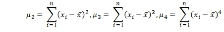
From a computer processing standpoint, however, they pose a special challenge in that they require the calculation of the difference between each element in the data set and the average of the data set implying two passes through the data: one to calculate the average and another to calculate the differences. In terms of a windowing-type function, this implies holding all the elements in memory and recalculating every time a new row is added to the resultant table. This would be painfully slow and would, in fact, represent at least the same overhead as doing a self-join.
Thankfully, there are single-pass algorithms available that allow for rapid, numerically stable calculations of each of the central moments.
Let’s look at what this means. First, let’s put some data into a table.
SELECT *
INTO #m
FROM (VALUES
(1,102),(2,142),(3,110),(4,110),(5,96),(6,101),(7,99),(8,96),(9,96),(10,126),(11,98),(12,105),(13,108),(14,126),(15,72),(16,114),(17,111),(18,100),(19,118),(20,84)
)n(rn,x)
Prior to SQL Server 2012 to calculate the running population variance you would have to use what is known as a self-join, which would look something like this.
SELECT m1.x
,VARP(m2.x) as VAR_P
FROM #m m1
JOIN #m m2
ON m2.rn <= m1.rn
GROUP BY m1.x, m1.rn
ORDER BY m1.rn
This produces the following result.
x VAR_P
----------- ----------------------
102 0
142 400
110 298.666666666667
110 236
96 252.8
101 227.472222222221
99 210.244897959184
96 201.25
96 190.83950617284
126 208.560000000001
98 197.537190082644
105 181.354166666667
108 167.514792899409
126 179.882653061224
72 249.493333333333
114 237.83984375
111 225.065743944637
100 214.83950617284
118 210.448753462603
84 224.710000000001
SQL Server 2012 offers a significant improvement over this, by eliminating the need for a self-join. Thus, the same result can be achieved in SQL Server 2012 using the following syntax.
SELECT x
,VARP(x) OVER (ORDER BY rn) as VAR_P
FROM #m
ORDER BY rn
Which is obviously much simpler and much less computationally intensive than the self-join. This produces the following result.
x VAR_P
----------- ----------------------
102 0
142 400
110 298.666666666667
110 236
96 252.8
101 227.472222222221
99 210.244897959184
96 201.25
96 190.83950617284
126 208.560000000001
98 197.537190082644
105 181.354166666667
108 167.514792899409
126 179.882653061224
72 249.493333333333
114 237.83984375
111 225.065743944637
100 214.83950617284
118 210.448753462603
84 224.710000000001
Of course, if you are not a SQL Server 2012 user, this syntax is not available to you unless you use the XLeratorDB/windowing library. You can now calculate the running population variance with a TSQL statement that looks like this.
SELECT x
,wct.RunningVARP(x, ROW_NUMBER() OVER (ORDER BY rn), NULL) as VAR_P
FROM #m
ORDER BY rn
This produces the following result.
x VAR_P
----------- ----------------------
102 0
142 400
110 298.666666666667
110 236
96 252.8
101 227.472222222222
99 210.244897959184
96 201.25
96 190.839506172839
126 208.56
98 197.537190082645
105 181.354166666667
108 167.514792899408
126 179.882653061225
72 249.493333333333
114 237.83984375
111 225.065743944637
100 214.839506172839
118 210.448753462604
84 224.71
Obviously, XLeratorDB takes advantage of the windowing capabilities of the ROW_NUMBER() function in SQL Server 2005 and above to provide this capability.
In this graph, we see that as the dataset grows, the processing time increases exponentially for the self-join whereas the windowing functions are more or less unaffacted.
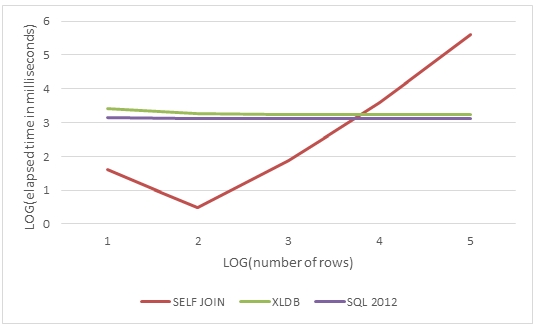
It is interesting to note that the self-join is actually somewhat faster for a small number of rows (<10,000) than using the windowing functions.
However, there is an additional advantage to using the XLeratorDB functions: numeric stability. The SQL Server central tendency functions are numerically unstable. Let’s look at what that means in the following example.
SELECT rn
,CAST(x as float) as x
,VARP(x) OVER (ORDER BY rn) as VAR_P
FROM (VALUES
(1,900.000001580507),
(2,900.000003161014),
(3,900.000000948304),
(4,900.000001580507),
(5,900.000003161014),
(6,900.00000118538),
(7,900.000001896608),
(8,900.00000237076)
)n(rn,x)
This produces the following result.
rn x VAR_P
----------- ---------------------- ----------------------
1 900.000001580507 0
2 900.000003161014 0
3 900.000000948304 0
4 900.000001580507 0
5 900.000003161014 0
6 900.00000118538 0
7 900.000001896608 0
8 900.00000237076 0
While the population variance is small it is not zero. Here’s what the results look like using the XLeratorBD function.
SELECT rn
,CAST(x as float) as x
,wct.RunningVARP(x,ROW_NUMBER() OVER (ORDER BY rn), NULL) as VAR_P
FROM (VALUES
(1,900.000001580507),
(2,900.000003161014),
(3,900.000000948304),
(4,900.000001580507),
(5,900.000003161014),
(6,900.00000118538),
(7,900.000001896608),
(8,900.00000237076)
)n(rn,x)
This produces the following result.
rn x VAR_P
----------- ---------------------- ----------------------
1 900.000001580507 0
2 900.000003161014 6.24500540873906E-13
3 900.000000948304 8.6597425224703E-13
4 900.000001580507 6.68215689240038E-13
5 900.000003161014 8.23341639369267E-13
6 900.00000118538 7.98840428231102E-13
7 900.000001896608 6.84911544100513E-13
8 900.00000237076 6.20499911840382E-13
The differences become more pronounced in the calculation of standard deviation (which is the square root of the variance).
SELECT rn
,CAST(x as float) as x
,STDEVP(x) OVER (ORDER BY rn) as [SQL SERVER STDEV_P]
,wct.RunningSTDEVP(x,ROW_NUMBER() OVER (ORDER BY rn), NULL) as [XLDB STDEV_P]
FROM (VALUES
(1,900.000001580507),
(2,900.000003161014),
(3,900.000000948304),
(4,900.000001580507),
(5,900.000003161014),
(6,900.00000118538),
(7,900.000001896608),
(8,900.00000237076)
)n(rn,x)
This produces the following result.
rn x SQL SERVER STDEV_P XLDB STDEV_P
----------- ---------------------- ---------------------- ----------------------
1 900.000001580507 0 0
2 900.000003161014 0 7.90253466220747E-07
3 900.000000948304 0 9.30577375744237E-07
4 900.000001580507 0 8.17444609279453E-07
5 900.000003161014 0 9.07381749524018E-07
6 900.00000118538 0 8.93778735611394E-07
7 900.000001896608 0 8.27593827973912E-07
8 900.00000237076 0 7.87718167773464E-07
As you can see, SQL Server 2012 has produced a population standard deviation of zero. While the standard deviation is small, it is clearly not zero. We have previously written about this problem in the SQL Server aggregate functions (see one-pass or two), but it’s surprising that the problem persists in SQL Server 2012.We have taken the same care to assure numerical stability in the calculation of kurtosis and skewness, both in our implementation of the aggregates and in the windowing version. SQL Server does not provide built-in functions for kurtosis and skewness.
The Sharpe ratio measures the ratio between the mean difference and the sample standard deviation of the differences for an investment return and a risk-free rate. It is very similar to Cohen’s D which may be used to measure the effect size in Student’s t test. It is also similar to the Information ratio, with the exception that the Information ratio compares investment returns to the return on a benchmark rather than to the risk-free rate. Since Sharpe, Information, and t test are so closely related we have created windowing versions of all three.
The Sharpe and Information ratio implementations allow you to use prices or returns as input into the function, though consistency is required in the window. In other words, you cannot switch to prices from returns half-way through the window. We have also implemented an exact flag, which when true will have the function return a NULL when the actual window size is smaller than the specified window size. In other words, if you want to do a 36-month rolling window of the Sharpe ratio, you have the ability to specify whether or not you want a non-NULL value returned when there are less than 36 rows in the window (which will usually be at the beginning of the data set).
The Sharpe ratio implementation is based on Sharpe’s 1994 formula and is arithmetically the same as the Information ratio. The only difference between the functions is that the Information ratio will calculate benchmark return from prices if the prices flag is set to true, whereas the Sharpe ratio always treats the risk-free rate as a rate and never as a price.
The TTEST windowing functions support the paired, equal variance and unequal variance tests. The paired t test requires that the both columns passed into the function be non-NULL to be included in the calculation. The equal and unequal variance tests simply require that one of the columns not be NULL.
For more information about these functions and all of our windowing functions, see the full windowing documentation.
Whether you are using SQL Server 2005, 2008, or 2012, we think that you will find these functions useful. If there are other functions you would like to see, please contact us at support@westclintech.com.