New functions for pricing American and European options in SQL Server
Sep
17
Written by:
Charles Flock
9/17/2012 8:21 PM

With the release of our newest library of functions, XLeratorDB/financial-options, you have the ability to calculate the price and Greeks for American and European options in SQL Server 2005, 2008, and 2012. This release includes the Black-Scholes-Merton pricing formula, the Bjerksund & Stensland 2002 American approximation, and binomial trees for American and European options. It also includes calculation of the implied volatility and some table-valued functions and stored procedures for analyzing the price and P&L impacts of changes in the underlying asset price, the volatility, the risk free rate, and time decay.
XLeratorDB/financial-options is our newest library of functions written specifically for SQL Server. It contains 8 new scalar functions for calculating the price and Greeks of American and European options; 6 new table-valued functions, including 3 that let you calculate all price and Greeks at the same time (which is much more efficient than doing them separately), 2 for analyzing how things like time decay, changes in price, changes in volatility, and changes in rates affect the price, the Greeks, or P&L, and one that shows all the nodes in the binomial tree for an American or European option .
XLeratorDB/financial-options, like the other XLeratorDB modules, stands alone (you don’t need any other XLeratorDB modules for it to work). However, you can combine it with the other modules (finance, statistics, math, engineering, and strings) to come up with a solution that is best for you. XLeratorDB/financial-options is priced at USD 599.99 per server. For more information about pricing and licensing terms, follow this link.
We have also included the XLeratorDB/financial-options functions in XLeratorDB/suite-plus, which is a library of all the functions, available for USD 1,499.99 and includes over 550 financial, statistical, and math functions written expressly for SQL Server.
New scalar functions
The new scalar functions are:
The BlackScholesMerton function is an implementation of the Generalized Black-Scholes-Merton option pricing formula. The general form of the function in a T-SQL statement is:
SELECT wct.BlackScholesMerton(z,S,K,T,r,d,s,rv)
Where
Z identifies the option as a put (P) or a call (C).
S the price of the underlying asset
K the strike price of the option
T the time to expiration in years
r the continuously compounded risk-free rate of return
d the continuously compounded dividend rate
s the volatility of the relative price change of the underlying asset
rv the value to be returned by the function (Price, Delta, Gamma, Theta, Lambda, Vega, or Rho)
This model can be used to price European options on stocks, stocks paying a continuous dividend yield, options on futures, and currency options.
BlackScholesMerton is a closed-form solution both in the calculation of the theoretical value of the option (Price) and in the calculation of the Greeks (Delta, Gamma, Theta, Lambda, Vega, or Rho). Thus, it performs quite well in SQL Server. In our test environment, using SQL Server 2008 R2, on a 64-bit Windows Server 2008 R2 machine, with 4GB of RAM and a 2.5 gHz Pentium dual core processor, we can price 10,000 options in about 990 milliseconds; about 10,000 a second. Your performance may differ based upon machine and software configurations.
BlackScholesMertonIV calculates the implied volatility of a European option. Implied volatility is calculated when you know the price of the option, and are looking for a value for volatility (s) such that when it is plugged into BlackScholesMerton it will return the input price. In SQL terms, we could define the implied volatility as the value that sets this statement equal to zero.
SELECT wct.BlackScholesMerton(z, S, K, T, r, d, wct.BlackScholesMertonIV(z, S, K, T, r, d, @price), 'P') - @price
It is important to note that the implied volatility is not necessarily a unique solution. It is possible to have many values of volatility that return the same price.
There is no closed form solution for implied volatility, so we solve it through iteration using a combined Newton-Raphson and bisection technique. In our test environment (described above) it takes about 4,020 milliseconds to calculate the implied volatility on 10,000 options; about 2,500 a second.
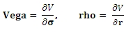
BjerksundStensland is an implementation of the Bjerksund and Stensland (2002) approximation and can be used to price American options on stocks, futures, and currencies. Like BlacksScholesMerton, it provides a closed form solution for the calculation of the theoretical value of an option. However, the Greeks are calculated as the first or second derivative of the price. For example, Delta is calculated as the first derivative of value of the option (V) with respect to the underlying price (S). So

The derivatives are calculated using a centered difference approximation. The calling structure for BjerksundStensland is the same as for BlackScholesMerton.
SELECT wct.BjerksundStensland(z,S,K,T,r,d,s,rv)
In our test environment, the calculation of Price using BjerksundStensland averaged 11,190 milliseconds per 10,000 rows, or slightly more than 11 seconds for 10,000 rows. The calculation of delta averaged 22,271 milliseconds pre 10,000 rows, or slightly more than 22 seconds for 10,000 rows. This is because the calculation of the first derivative of the function requires that we call the function twice and the first derivative take approximately twice the time. Gamma, which is a second derivative Greek, averaged 35,903 milliseconds per 10,000 rows, or about 36 second for 10,000. The calculation of the second derivative requires that we call the function three times, hence the increased processing time.
BjerksundStensland IV calculates the implied volatility of an American option. As with BlackScholesMertonIV, implied volatility is calculated knowing the price of the option and looking for a value for volatility (s) such that when it is plugged into BjerksundStensland it will return that price. In SQL terms, we could define the implied volatility as the value that sets this statement equal to zero.
SELECT wct.BjerksundStensland(z, S, K, T, r, d, wct.BjerksundStenslandIV(z, S, K, T, r, d, @price), 'P') - @price
Once again, it is important to note that the implied volatility is not necessarily a unique solution. It is possible to have many values of volatility that return the same price.
There is no closed form solution for implied volatility, so we solve it through iteration using a combined Newton-Raphson and bisection technique. In our test environment (described above) it takes about 219,723 milliseconds to calculate the implied volatility on 10,000 options; about 46 a second.
BinomialEuro is an implementation of the Cox, Ross, Rubenstein binomial method and can be used to price most European Options. BinomialEuro is a numerical method for calculating the price and Greeks and performance and accuracy are both affected by the number of steps in the binomial tree. Some of the Greeks can be calculated directly from the tree structure, so there is no additional overhead required in their calculation. However the calculation of vega and rho both require calculation of the first derivative, which we do by finite difference using a forward difference approximation. So
The calling structure for BinomialEuro is similar to BjerksundStensland and BlackScholesMerton, with addition of a parameter specifying the number of steps in the binomial tree.
SELECT wct.BinomialEuro(z,S,K,T,r,d,s,n,rv)
In our test environment, the calculation of price using BinomialEuro with the number of steps set to 50, averaged 10,256 milliseconds per 10,000 rows, or slightly more than 10 seconds for 10,000 rows. When we doubled the number of steps to 100, the price calculation averaged 36,575 milliseconds, or about 37 seconds per 10,000 rows. This is what we expect, as the number of nodes in the binomial tree increases exponentially with the number of steps giving rise to concomitant increase in the processing time.
As expected, given that its value can be calculated directly from a node on the binomial tree, the processing time for the calculation of delta is roughly equivalent to that of the price calculation: 10,634 milliseconds at 50 steps and 35,505 milliseconds for 100 steps with the same 10,000 rows of data. The calculation of vega, which cannot be observed directly from the binomial tree, took roughly twice as long: 20,767 milliseconds at 50 steps and 67,445 milliseconds for 100 steps.
BinomialEuroIV, as with all the implied volatility functions, calculates the implied volatility using the price of the option and looking for a value for volatility (s) such that when it is plugged into BinomialEuro it will return that price. In SQL terms, we could define the implied volatility as the value that sets this statement equal to zero.
SELECT wct.BinomialEuro(z, S, K, T, r, d, wct.BinomialEuroIV(z, S, K, T, r, d, n, @price), n, 'P') - @price
As always, it is important to note that the implied volatility is not necessarily a unique solution. It is possible to have many values of volatility that return the same price.
There is no closed form solution for implied volatility, so we solve it through iteration using a combined Newton-Raphson and bisection technique. In our test environment (described above), setting the number of steps to 50, it takes about 97,408 milliseconds to calculate the implied volatility on 10,000 options; about 103 a second. When you set the number of steps to 100, the average is 362,825 milliseconds; about 28 a second.
BinomialAmerican is very similar to BinomialEuro and is used for calculating the price and Greeks of American options. Except for the function name, the calling structure is the same.
SELECT wct.BinomialAmerican(z,S,K,T,r,d,s,n,rv)
In our test environment, the calculation of price with the number of steps set to 50, using BinomialAmerican averaged 15,586 milliseconds per 10,000 rows, or slightly more than 15 seconds for 10,000 rows. When we doubled the number of steps to 100, the price calculation averaged 61,052 milliseconds, or about 61 seconds per 10,000 rows. The corresponding numbers for delta are 15,978 milliseconds for 50 steps and 59,428 milliseconds for 100 steps.
As expected, the calculation of vega, which requires two calculations of the price, takes 32,871 milliseconds at 50 steps and 117,125 milliseconds at 100 steps.
BinomialAmericanIV works just like BinomialEuroIV in that it is trying to find a value for volatility such that the following expression is approximately zero.
SELECT wct.BinomialAmerican(z, S, K, T, r, d, wct.BinomialAmericanIV(z, S, K, T, r, d, n, @price), n, 'P') - @price
As always, it is important to note that the implied volatility is not necessarily a unique solution. It is possible to have many values of volatility that return the same price.
There is no closed form solution for implied volatility, so we solve it through iteration using a combined Newton-Raphson and bisection technique. In our test environment (described above), setting the number of steps to 50, it takes about 137,688 milliseconds to calculate the implied volatility on 10,000 options; about 73 a second. When you set the number of steps to 100, the average is 530,953 milliseconds; about 19 a second.
New table-valued functions
The new table-valued functions are:
The BlackScholesMertonPriceNGreeks table-valued function returns the price, delta, lambda, gamma, vega, rho, and theta for a European option. Instead of having to call BlackScholesMerton multiple times for each option, you can simply invoke BlackScholesMertonPriceNGreeks and select the columns that you want returned. You can enter this:
SELECT a.recno
,k.*
FROM <table> a
CROSS APPLY wct.BlackScholesMertonPriceNGreeks(z,S,K,T,r,d,s) k
instead of entering this.
SELECT a.recno
,wct.BlackScholesMerton(z,S,K,T,r,d,s,'P') as Price
,wct.BlackScholesMerton(z,S,K,T,r,d,s,'D') as Delta
,wct.BlackScholesMerton(z,S,K,T,r,d,s,'L') as Lambda
,wct.BlackScholesMerton(z,S,K,T,r,d,s,'G') as Gamma
,wct.BlackScholesMerton(z,S,K,T,r,d,s,'V') as Vega
,wct.BlackScholesMerton(z,S,K,T,r,d,s,'R') as Rho
,wct.BlackScholesMerton(z,S,K,T,r,d,s,'T') as Theta
FROM <table> a
The table-valued function should provide better performance than calling the scalar function multiple times. In our test environment, the table-valued function would return the price and greeks for 10,000 rows in 1,135 milliseconds or about 7,600 rows per second. This represents a 675 percent improvement in pefroemance over using the the scalar function 7 times for each row.
The BjerksundStenslandPriceNGreeks table-valued function returns the price, delta, lambda, gamma, vega, rho, and theta for an American option. Instead of having to call BjerksundStensland multiple times for each option, you can simply invoke BjerksundStenslandPriceNGreeks and select the columns that you want returned. You can enter this:
SELECT a.recno
,k.*
FROM <table> a
CROSS APPLY wct.BjerksundStenslandPriceNGreeks(z,S,K,T,r,d,s) k
instead of entering this.
SELECT a.recno
,wct.BjerksundStensland (z,S,K,T,r,d,s,'P') as Price
,wct.BjerksundStensland (z,S,K,T,r,d,s,'D') as Delta
,wct.BjerksundStensland (z,S,K,T,r,d,s,'L') as Lambda
,wct.BjerksundStensland (z,S,K,T,r,d,s,'G') as Gamma
,wct.BjerksundStensland (z,S,K,T,r,d,s,'V') as Vega
,wct.BjerksundStensland (z,S,K,T,r,d,s,'R') as Rho
,wct.BjerksundStensland (z,S,K,T,r,d,s,'T') as Theta
FROM <table> a
The table-valued function should provide better performance than calling the scalar function multiple times. In our test environment, the table-valued function would return the price and greeks for 10,000 rows in 111,990 milliseconds or about 89 rows per second. This represents a 59% improvement in perfromance over calling the scalar function 7 times for each row.
The BinomialPriceNGreeks table-valued function returns the price, delta, lambda, gamma, vega, rho, and theta for European or American options. Instead of having to call BinomialAmerican or BinomialEuro multiple times for each option, you can simply invoke BinomialPriceNGreeks and select the columns that you want returned. You can enter this:
SELECT a.recno
,k.*
FROM <table> a
CROSS APPLY wct.BinomialPriceNGreeks(z,S,K,T,r,d,s,n,'A') k
instead of entering this.
SELECT a.recno
,wct.BinomialAmerican(z,S,K,T,r,d,s,n,'P') as Price
,wct.BinomialAmerican(z,S,K,T,r,d,s,n,'D') as Delta
,wct.BinomialAmerican(z,S,K,T,r,d,s,n,'L') as Lambda
,wct.BinomialAmerican(z,S,K,T,r,d,s,n,'G') as Gamma
,wct.BinomialAmerican(z,S,K,T,r,d,s,n,'V') as Vega
,wct.BinomialAmerican(z,S,K,T,r,d,s,n,'R') as Rho
,wct.BinomialAmerican(z,S,K,T,r,d,s,n,'T') as Theta
FROM <table> a
For European options, simply change the 'A' to an 'E' in BinomialPriceNGreeks.
The following table summarizes the differences in performance.
|
Functions
|
Steps
|
Time
(milliseconds)
|
Rows /
second
|
scalar /
TVF
|
|
BinomialAmerican
|
50
|
154,454.00
|
65
|
|
|
BinomialAmericanPriceNGreeks
|
50
|
43,548.67
|
230
|
255%
|
|
BinomialEuro
|
50
|
89,452.67
|
112
|
|
|
BinomialEuroPriceNGreeks
|
50
|
30,026.33
|
333
|
198%
|
|
BinomialAmerican
|
100
|
538,872.00
|
19
|
|
|
BinomialAmericanPriceNGreeks
|
100
|
159,997.33
|
63
|
237%
|
|
BinomialEuro
|
100
|
317,127.33
|
32
|
|
|
BinomialEuroPriceNGreeks
|
100
|
105,963.00
|
94
|
199%
|
|
|
|
|
|
The table-valued function BinomialTree shows all the nodes in the Binomial Tree calculation for an American or European Option. Usually when discussing the nodes on the binomial tree you end up with a diagram that looks something like this:
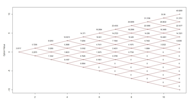
While this might be interesting to look at, we can’t really extract any of the data in the diagram. However, with the BinomialTree table-valued function, it is now possible to return a third-normal form representation of the nodes. Here’s the SQL, using the same data that was used to create the diagram above.
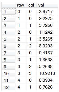
SELECT row, col, cast(val as money) as val
FROM wct.BinomialTree('C',99.5,100,.249315,.002,.01,.22,10,'E')
Here are the first few rows of the result.
We can use the PIVOT function to return a lower triangular matrix representation of the nodes on the binomial tree.
SELECT row,[0],[1],[2],[3],[4],[5],[6],[7],[8],[9],[10]
FROM (
SELECT row, col, cast(val as money) as val
FROM wct.BinomialTree('C',99.5,100,.249315,.002,.01,.22,10,'E')
) d
PIVOT(sum(val) for col in([0],[1],[2],[3],[4],[5],[6],[7],[8],[9],[10])) as P
This produces the following result.
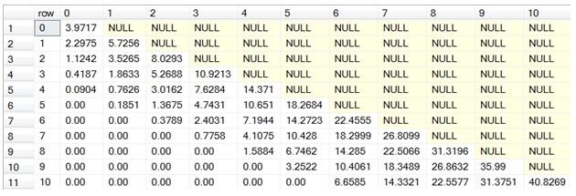
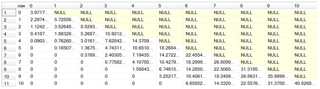
The value of the (0,0) node is the price of the option, in this case 3.9717.
You can also use the sp_BinomialTree stored procedure to automatically PIVOT the binomial tree.
EXECUTE wct.sp_BinomialTree'C',99.5,100,.249315,.002,.01,.22,10,'E'
This produces the following result.
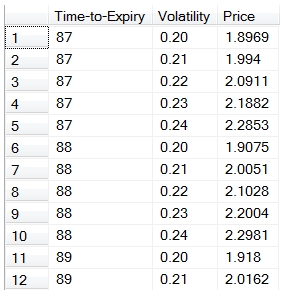
The table-valued function OptionMatrix allows you to evaluate how changes in two of the input values affecting the value returned by the function. For example, let’s say you wanted to know how changes in the volatility and changes in the time to expiry would affect the price of an option. Without the OptionMatrix function you might have to construct SQL that looks something like this.
SELECT n.t as [Time-to-Expiry]
,m.v as [Volatility]
,cast(wct.BlackScholesMerton('C',50,50,n.t/cast(365 as float),.002,.01,m.v,'P') as money) as Price
FROM (VALUES (92),(91),(90),(89),(88),(87)) n(t)
CROSS APPLY(VALUES (.24),(.23),(.22),(.21),(.20))m(v)
ORDER BY 1, 2
Here are the first few rows of the result set.
With the table-valued function, the SQL is simplified into this.
SELECT row as [Time-to-Expiry]
,col as [Volatility]
,CAST(val as money) as Price
FROM wct.OptionMatrix('C',50,50,92/cast(365 as float),.002,.01,.22,'P','E','VOL',.01,2,'TIME',1,5)
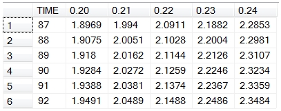
Of course, many people we will want to see this in spreadsheet format, so you might end up having to PIVOT the result set. The sp_OptionMatrix stored procedure will do this for you automatically (no need to figure out the PIVOT values ahead of time), with an almost identical calling structure as the table-valued function.
EXECUTE wct.sp_OptionMatrix'C',50,50,0.2520548,.002,.01,.22,'P','E','TIME',1,5,'VOL',.01,2,1,4
This produces the following result.
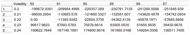
The table-valued function OptionPLMatrix is similar to the OptionMatrix function, in that it allows you to analyze the impact of changes to two inputs into the theoretical value of the option. It differs in that it is only concerned with the theoretical value of the option and actually calculates the difference between the theoretical value of the option given the initial input parameters and the theoretical value of the option given the new parameters, giving you an indication of the profit (or loss) as those parameters change.
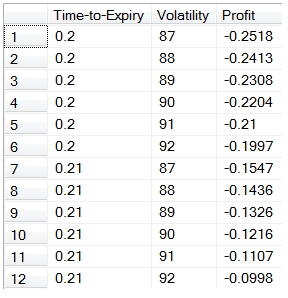
Using the same parameters as the previous example, we can see how changes in time and volatility can affect the profit on the option.
SELECT row as [Time-to-Expiry]
,col as [Volatility]
,CAST(val as money) as Profit
FROM wct.OptionPLMatrix('C',50,50,92/cast(365 as float),.002,.01,.22,'E','VOL',.01,2,'TIME',1,5)
Here are the first few rows of the result set.
In this example, we will take the change in price and multiply it by the notional value of the position (1,000,000) and PIVOT the results into a matrix format.
SELECT [Volatility],[92],[91],[90],[89],[88],[87]
FROM (
SELECT row as [Volatility]
,col as [Time-to-Expiry]
,CAST(val * 1000000 as money) as Profit
FROM wct.OptionPLMatrix('C',50,50,92/cast(365 as float),.002,.01,.22,'E','VOL',.01,2,'TIME',1,5)
) d
PIVOT(sum(Profit) for [Time-to-Expiry] in([92],[91],[90],[89],[88],[87])) as P
This produces the following result.
You could also use the sp_OptionPLMatrix function to automatically pivot the results for you.
DECLARE @t as float = 92/cast(365 as float)
EXEC wct.sp_OptionPLMatrix 'C',50,50,@t,.002,.01,.22,'E','VOL',.01,2,'TIME',1,5,1000000,2
This produces the following result.
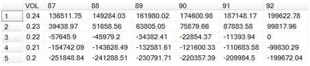
Notice that the stored procedure not only automatically created the PIVOT for you, but it orders the results in such a way the lowest left hand cell contains the biggest loss (where the volatility is 0.2 and the days to expiry is 87) and upmost right hand cell (where the volatility is 0.24 and the days to expiry is 92) contains the biggest gain.
New stored procedures
The new stored procedures are
Examples of these stored procedures can be found with the table-valued functions. These three stored procedures take the output of the table-valued functions and convert them into a matrix or spreadsheet style presentation, which may be easier for end-users to use.
The sp_BinomialTree stored procedure reformats that output of the table-value function BinomialTree into a matrix or spreadsheet format where result is a lower triangular matrix representation of the nodes in the binomial tree. Its calling structure is the same as the table value function, though it’s important to remember that stored procedures do not evaluate functions as input parameter; you can only pass in values or variables.
The sp_OptionPLMatrix stored procedure calls the OptionPLMatrix table-valued function and pivots the results into a matrix format. It includes two fields that are not part of the table-valued function: a notional amount and the number of decimals. These parameters allow you to calculate a monetary value for the change in the theoretical value of the option and display the results to the specified number of decimal places. It also sorts the results in such a way that the least monetary value will appear in the bottom left hand corner of the result set and the greatest monetary value will appear in the top right corner of the result set.
The sp_OptionsMatrix stored procedure calls the OptionMatrix table-valued function and pivots the results into a matrix format. It also includes a notional value and decimals as input parameters allowing you to convert the theoretical value of the option or any of the Greeks into a monetary value.
You can find out more about these functions by going to the documentation pages. You can try any of these functions out by downloading the 15-day free trial. If there is anything that you would like to see added, just send us an e-mail at support@westclintech.com.