Multiple linear regression in SQL Server
Mar
1
Written by:
Charles Flock
3/1/2012 3:33 PM

Using the LINEST function in SQL Server to do an Ordinary Least Squares calculation and the TRENDMX function to estimate housing prices.
A few weeks ago I was reading an article in the Wall Street Journal about how the real estate web site Zillow comes up with a value for a house. The article didn’t go into Zillow’s methodology, but it immediately occurred to me that this was a problem that was tailor-made for ordinary least squares, which is implemented in XLeratorDB in the LINEST and TRENDMX functions. This will let us calculate the coefficients for the line that best fits the x- and y-values that are in our database and calculate a value based on new x-values which are passed into the function.
The equation used in the OLS solutions where a y-intercept is calculated is

Without making this too complicated, this simply means that given multiple rows of x-values (in the range xn to x1, where n is the number of columns containing x-values) and a vector of y-values (meaning that each row only has one y-value), we can calculate mn to m0 where m is multiplied by the corresponding x-value and m0 is the y-intercept. We have the option of calculating the y-intercept or not.
Let’s look at a very simple example.
|
y
|
x1
|
x2
|
x3
|
|
-4
|
2
|
-1
|
1
|
|
2
|
1
|
-5
|
2
|
|
5
|
-3
|
1
|
-4
|
|
-1
|
1
|
-1
|
1
|
What we will do using the LINEST function, is find the best m-values in the equation:
y = m1x1 + m2x2 + m3x3
What’s the definition of the best value? The best values are the ones that minimize the sum of squared vertical distances between the observed responses in the data and the responses predicted by the linear approximation. In other words, the values for m will create a line that best fits the data in the table.
The following T-SQL (in SQL Server 2008 syntax) will put our data into a temporary table and return the m-values by invoking the LINEST function.
SELECT *
INTO #x
FROM (VALUES
(-4,2,-1,1),
(2,1,-5,2),
(5,-3,1,-4),
(-1,1,-1,1)
) n(y,x1,x2,x3)
SELECT *
FROM wct.LINEST(
'#x' --Table Name
,'*' --Column Names
,'' --Grouped Column Name
,NULL --Grouped Column Value
,1 --Y Column Number
,'False' --Y Intercept
)
This produces the following result.
Just like the EXCEL function of the same name, the XLeratorDB LINEST function returns the m-values, the standard error of the m-values (se), the coefficient of determination (rsq), the standard error of the y estimate (sey), the F-observed value (F), the degrees of freedom (df), the regression sum of squares (ss_req) and the residual sum of squares (ss_resid). For more information about these values, please refer to the LINEST documentation. For the purposes of this article, we are only going to concern ourselves with the m-values.
Our results are telling us that the equation that best fits the values in our table is the following:
y = -2.57142857142857(x1) - 0.719047619047619(x2) + 0.509523809523811(x3)
If we wanted to calculate using a y-intercept, we simply change the parameter in the LINEST function.
SELECT *
FROM wct.LINEST(
'#x' --Table Name
,'*' --Column Names
,'' --Grouped Column Name
,NULL --Grouped Column Value
,1 --Y Column Number
,'True' --Y Intercept
)
This produces the following result.
Making our equation:
y = 0.5 – 3.0(x1) - 0.5 (x2) + 1(x3)
Since we see that r2 (rsq) is 1, we know that this equation perfectly fits the date in our data set. Given this information, we can now calculate a new y-value when given new x-values. One way to do that would be to store the LINEST values and use the stored coefficients every time we are given new x-values.
However, we will find that it is much easier to use the TRENDMX function to calculate the new y-value. Assuming that none of our data have changed, let’s calculate a new y-value when x1 = 1, x2 = 2, and x3 = 4.
SELECT wct.TRENDMX(
'#x' --Table Name
,'*' --Column Names
,'' --Grouped Column Name
,NULL --Grouped Column Value
,1 --Y Column Number
,'1,2,4' --New x-values
,'True' --Y Intercept
) [New y]
This produces the following result.
Let’s take these two functions, LINEST and TRENDMX, and apply them to the problem of coming up with a value for a home based on some parameters. For purposes of this example, I created the following table:
CREATE TABLE [dbo].[HOMES](
[schooldistrict] [nvarchar](50) NOT NULL,
[lot] [float] NOT NULL,
[lotsize] [float] NOT NULL,
[housesize] [float] NOT NULL,
[age] [float] NOT NULL,
[bedrooms] [float] NOT NULL,
[bathrooms] [float] NOT NULL,
[distancefromriver] [float] NOT NULL,
[valuation] [float] NOT NULL,
CONSTRAINT [PK_HOMES] PRIMARY KEY CLUSTERED
(
[schooldistrict] ASC,
[lot] ASC
)
)
Which captures the following information about a house:
· the school district in which the property is located,
· the lot number, which is a way of uniquely identifying a lot within a school district.
· the size of the lot (in square feet),
· the size of the house (in square feet),
· the age of the house (in years),
· the number of bedrooms in the house,
· the number of bathrooms in the house,
· the distance from the river (in feet), and
· the value of the house
I then put 100,000 rows of data into my table, spread across 25 school districts. This data is completely made up and is only being used here to demonstrate multiple linear regression in SQL Server. Your data will be different and the characteristics that you want to capture and perform the regression analysis on will almost certainly be different. I selected these purely for demonstration purposes. If you want a copy of the data that I used in this example, you can get it be clicking here.
We can run the following SELECT statement to analyze the data.
SELECT t as [School District], k.*
FROM (SELECT distinct schooldistrict from HOMES) n(t)
CROSS APPLY wct.LINEST(
'HOMES' --Table name
,'valuation, lotsize, housesize, age, bedrooms, bathrooms, distancefromriver' --Column Names
,'schooldistrict' --Grouped Column Name
,n.t --Grouped Column Value
,1 --Y Column Number
,'TRUE' --Y Intercept
) k
where stat_name = 'm'
Here are the first few rows in the resultant table.
While this has returned the coefficients m0 though m6 for each of the school districts, it’s a little hard to read. Let’s run the following SQL, which provides a description for each of the coefficients and uses the PIVOT function to put the results in an easy-to-read spreadsheet format.
SELECT [School District]
,ROUND([6], 2) as [Distance from river]
,ROUND([5], 2) as [Bathrooms]
,ROUND([4], 2) as [Bedrooms]
,ROUND([3], 2) as [Age]
,ROUND([2], 2) as [House size]
,ROUND([1], 2) as [Lot Size]
,ROUND([0], 2) as [y intercept]
FROM (
SELECT t as [School District], k.*
FROM (SELECT distinct schooldistrict from HOMES) n(t)
CROSS APPLY wct.LINEST('HOMES'
,'valuation, lotsize, housesize, age, bedrooms, bathrooms, distancefromriver'
,'schooldistrict'
,n.t
,1
,'TRUE'
) k
where stat_name = 'm'
) M PIVOT(
max(stat_val)
FOR IDX in([6],[5],[4],[3],[2],[1],[0])
) AS PVT
This produces the following result.
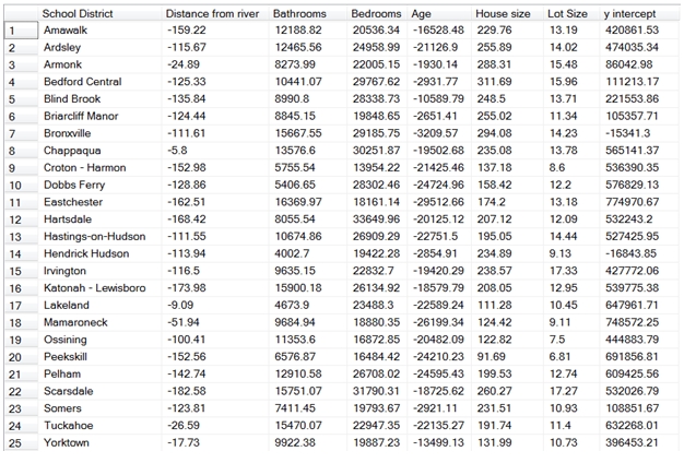
This makes it a little easier to interpret the results. Let’s look at row 10, which is a school district named Dobbs Ferry.
· For every additional foot that a house is from the river, its value declines by 128.86.
· For each additional bathroom, its value increases 5,406.65.
· For each additional bedroom, its value increases by 28,302.46.
· For each additional year in age, its value decreases 24,724.96.
· For each additional square foot in size, its value increases 158.42.
· For each additional square foot in lot size, its value increases 12.20.
· Finally, the y-intercept for Dobbs Ferry is 576,829.13, which represents the value of living in Dobbs Ferry not directly attributable to the coefficients that we have calculated.
Now that we have a model for the 25 school districts in our database, we might want to know how well the coefficients match the data. One statistic that we might want to look at is the r2 statistic. We can get that information with the following SELECT statement.
SELECT t as [School District]
, k.stat_val as [r-squared]
FROM (SELECT distinct schooldistrict from HOMES) n(t)
CROSS APPLY wct.LINEST(
'HOMES' --Table name
,'valuation, lotsize, housesize, age, bedrooms, bathrooms, distancefromriver' --Column Names
,'schooldistrict' --Grouped Column Name
,n.t --Grouped Column Value
,1 --Y Column Number
,'TRUE' --Y Intercept
) k
where stat_name = 'rsq'
This produces the following result.
All the r2 values are pretty close to 1, where 1 would mean that the coefficients are a perfect fit. For our purposes, we can assume that the coefficients provide a good enough fit, though there are certainly plenty of other analyses that you could do to make that determination.
Now we can come up with a few lines of SQL that will automatically estimate the price of a house based on the data in our database.
DECLARE @lotsize as float = 45000
DECLARE @housesize as float = 5000
DECLARE @age as float = 40
DECLARE @bedrooms as float = 4
DECLARE @bathrooms as float = 4
DECLARE @distancefromriver as float = 1239
DECLARE @schooldistrict as varchar(50) = 'Dobbs Ferry'
DECLARE @new_x as varchar(MAX)
SET @new_x = CAST(@lotsize as varchar) + CHAR(44)
SET @new_x = @new_x + CAST(@housesize as varchar) + CHAR(44)
SET @new_x = @new_x + CAST(@age as varchar) + CHAR(44)
SET @new_x = @new_x + CAST(@bedrooms as varchar) + CHAR(44)
SET @new_x = @new_x + CAST(@bathrooms as varchar) + CHAR(44)
SET @new_x = @new_x + CAST(@distancefromriver as varchar)
SELECT wct.TEXT(wct.TRENDMX('HOMES'
,'valuation, lotsize, housesize, age, bedrooms, bathrooms, distancefromriver'
,'schooldistrict'
,@schooldistrict
,1
,@new_x
,'True'
), '$#,###.00') as Estimate
This produces the following result.
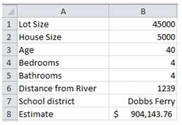
We have estimated that a 40-year old, 4-bedroom, 4-bathroom, 5,000 square foot house on a 45,000 square foot lot, 1,239 feet from the river in Dobbs Ferry is worth $904,143.76. We could change any of the parameters, including the school district, to come up with other estimates.
More than likely, however, we will not want to use SMS as our front-end. Since these functions are part of my SQL Server database, I can use any platform that can open a connection to the database as a front-end. Since I like to keep things nice and simple, here’s an example using VBA in EXCEL.
You can simply open a new workbook, hit alt + F11, insert a new module, and paste the following code into the VBA editor.
Go to Tools, References, and click the checkbox for Microsoft ActiveX Data Objects 6.0 Library.
The GetStrConn() function simply creates a string with your credentials to connect to the database. You will need to provide the connection string particular to your environment and you could even just set StrConn equal to the appropriate value without calling a separate function. The Zestimate function connects to the database, and based on the inputs provided to the function, returns a value to the cell where the formula is entered.
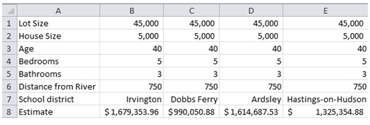
In Sheet1 I entered the following labels and formula.
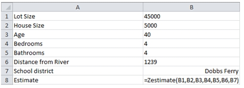
Which returns the following result.
Now, it is very easy to make changes and look at the results. Let’s see what the same house would cost in Irvington.
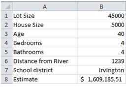
In fact, now it becomes quite easy to do side-by-side comparisons.
Remember, none of the data are in EXCEL. Everything is stored in the SQL Server database and none of the data move across the network. Our VBA function, instead of selecting the data, requests the database to do the calculation and return the result. The only thing that moves over the network is our SQL String and the result of the calculation. All-in-all, less than a kilobyte of data.
Is it possible that we could have just put all our data into EXCEL and used the EXCEL TREND function to do that calculation? Not really. While our example has only 100,000 rows of data, it will work exactly the same if there were a million rows or 10 million rows. And, since we are running on the database, the TRENDMX function is always using the latest data. It’s not really practical to think about putting this kind of volume into a spreadsheet. Additionally, there is no way to filter the data within the EXCEL functions, which rely exclusively on ranges for input. And, structured references don’t solve that problem, as new data are constantly being added to or updated on the database.
The following SQL, which I ran on my 32-bit laptop, gives us some information about the amount of time it takes the query to execute on the server.
SET STATISTICS TIME ON
SELECT wct.TRENDMX('HOMES'
,'valuation, lotsize, housesize, age, bedrooms, bathrooms, distancefromriver'
,'schooldistrict'
,'Irvington'
,1
,'45000,5000,40,5,3,750'
,'TRUE')
SET STATISTICS TIME OFF
This produces the following result.
Of course, your times will differ.
The beauty of this approach is that whenever new data are added to the HOMES table, the model is automatically recalibrated. And since it all happens on the server, there is no need to change the model in the presentation layer (in this case, EXCEL). There is also very little code in EXCEL. And, there is no data in EXCEL.
The LINEST and TRENDMX functions are great tools for analyzing your business data and for beginning to build your own predictive analytics. Having these functions on the database makes it simple.