Fast Multiple Linear Regression in SQL Server
Oct
7
Written by:
Charles Flock
10/7/2013 11:16 AM

In this article we talk about the XLeratorDB TRENDMX and LINEST functions and describe some techniques to turbo-charge your predictive analytics in SQL Server.
XLeratorDB users have known for years that they can use the TRENDMX function to predict outcomes based upon models with multiple columns of input. The scalar TRENDMX function works like the Excel TREND function for multiple linear regression. XLeratorDB also has an aggregate TREND function which calculates a predicted value based on a single column of x-values.
Let’s review how that works, based on an example in the Excel documentation for LINEST. In this example a developer randomly chooses a sample of 11 office buildings from a possible 1,500 office buildings and obtains the following data.
|
Floor Space
|
Offices
|
Entrances
|
Age
|
Assessed Value
|
|
2,310
|
2
|
2
|
20
|
142,000
|
|
2,333
|
2
|
2
|
12
|
144,000
|
|
2,356
|
3
|
1.5
|
33
|
151,000
|
|
2,379
|
3
|
2
|
43
|
150,000
|
|
2,402
|
2
|
3
|
53
|
139,000
|
|
2,425
|
4
|
2
|
23
|
169,000
|
|
2,448
|
2
|
1.5
|
99
|
126,000
|
|
2,471
|
2
|
2
|
34
|
142,900
|
|
2,494
|
3
|
3
|
23
|
163,000
|
|
2,517
|
4
|
4
|
55
|
169,000
|
|
2,540
|
2
|
3
|
22
|
149,000
|
Let’s put this data into a table. To simplify things we will call the column headings x1, x2, x3, x4, and y and I will add an identity column to keep track of the rows.
SELECT IDENTITY(int,1,1) as rn
,[Floor Space] as x1
,[Offices] as x2
,[Entrances] as x3
,[Age] as x4
,[Assessed Value] as y
INTO #L
FROM (VALUES
(2310,2,2,20,142000)
,(2333,2,2,12,144000)
,(2356,3,1.5,33,151000)
,(2379,3,2,43,150000)
,(2402,2,3,53,139000)
,(2425,4,2,23,169000)
,(2448,2,1.5,99,126000)
,(2471,2,2,34,142900)
,(2494,3,3,23,163000)
,(2517,4,4,55,169000)
,(2540,2,3,22,149000)
)n([Floor Space],[Offices],[Entrances],[Age],[Assessed Value])
This SQL produces the following table.
|
rn
|
x1
|
x2
|
x3
|
x4
|
y
|
|
1
|
2310
|
2
|
2
|
20
|
142000
|
|
2
|
2333
|
2
|
2
|
12
|
144000
|
|
3
|
2356
|
3
|
1.5
|
33
|
151000
|
|
4
|
2379
|
3
|
2
|
43
|
150000
|
|
5
|
2402
|
2
|
3
|
53
|
139000
|
|
6
|
2425
|
4
|
2
|
23
|
169000
|
|
7
|
2448
|
2
|
1.5
|
99
|
126000
|
|
8
|
2471
|
2
|
2
|
34
|
142900
|
|
9
|
2494
|
3
|
3
|
23
|
163000
|
|
10
|
2517
|
4
|
4
|
55
|
169000
|
|
11
|
2540
|
2
|
3
|
22
|
149000
|
Again, using the Excel example, if we wanted to estimate the assessed value (y) of an office building with 2500 square feet of office space (x1), 3 offices (x2), 2 entrances (x3), which is 25-years old (x4) we could simply enter the following SQL.
SELECT wct.TRENDMX('#L','y,x1,x2,x3,x4','',NULL,1,'2500,3,2,25','True') as [Predicted Value]
This produces the following result.
Predicted Value
----------------------
158261.095632605
Let’s make things a little more interesting. Let’s calculate the predicted for each row in the #L temp table and compare it to the actual assessed value. Again, this is pretty straightforward in terms of the TRENDMX function; we can just enter the following SQL.
SELECT rn
,y as [Assessed Value]
,wct.TRENDMX('#L','y,x1,x2,x3,x4','',NULL,1,'SELECT x1,x2,x3,x4 FROM #L WHERE rn = ' + cast(rn as varchar(max)),'True') as [Predicted Value]
FROM #L
The results look like this.
|
rn
|
Assessed Value
|
Predicted Value
|
|
1
|
142000
|
141650.65
|
|
2
|
144000
|
144160.299
|
|
3
|
151000
|
151130.233
|
|
4
|
150000
|
150700.219
|
|
5
|
139000
|
139017.042
|
|
6
|
169000
|
169186.234
|
|
7
|
126000
|
125683.82
|
|
8
|
142900
|
142821.593
|
|
9
|
163000
|
161116.932
|
|
10
|
169000
|
169340.074
|
|
11
|
149000
|
150092.905
|
While that’s very easy in terms of SQL, there is quite a bit of processing going on inside the TRENDMX function. For every row in the resultant table, the function executed dynamic SQL which returned the specified columns of the #L table. That data are then used in an ordinary least square calculation which returns the coefficients which are then used with the new x-values to calculate the predicted value.
Even though that calculation is done 11 times, the coefficients are the same for each row. This is true because the data are not dynamic—we are using the same data each time.
If we returned 100 rows then the calculation would be done 100 times; 1,000 rows, 1,000 times. For a small table like the one that we are dealing with here, the overhead isn’t too great, but if we were dealing with 25 variables, or 50 variables, or even 100 then we could be talking about considerable amounts of processing time.[1]
In situations like this, where we want to calculate many predicted values using the same coefficients, it is quite easy to use the LINEST function to calculate the coefficient once and then apply the coefficients once to the new x-values and achieve stunning increases in performance.
The following SQL will store the coefficients in a table called #coef.
SELECT idx, stat_val as m
INTO #coef
FROM wct.LINEST('#L','y,x1,x2,x3,x4','',NULL,1,'TRUE')
WHERE stat_name = 'm'
The #coef table contains that following values.
|
idx
|
m
|
|
0
|
52317.83
|
|
1
|
27.64139
|
|
2
|
12529.77
|
|
3
|
2553.211
|
|
4
|
-234.237
|
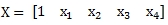
One complaint about the Excel LINEST function is that it stores the m-values in the opposite order of the new x-values. In other words, EXCEL returns the m-values as a vector in the following order:
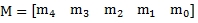
whereas the x-values are passed into the function in this order.[2]
What should then be a very straightforward calculation, 
can be (and is) extremely error-prone and tedious in Excel.[3]
However, that is not the case with XLeratorDB's LINEST function in SQL Server. In fact, since the coefficients are returned from the function in 3rd normal form, we don’t care at all as to how they are physically stored. We just join the appropriate x-values to the appropriate m-values and calculate the sum of the product which is quite simple.
But, first we have to take our x-values, which are stored in columns x1, x2, x3, and x4 and turn them into rows. This sounds an awful lot like the UNPIVOT function in SQL Server, but here is a very simple way to achieve the same result using CROSS APPLY. We will store the normalized new x-values in a temp table called #newx. We will use the x1, x2, x3, and x4 values from the #L table to populate the #newx table.
SELECT #L.rn
,n.idx
,n.x
INTO #newx
FROM #L
CROSS APPLY(VALUES (0,1),(1,x1),(2,x2),(3,x3),(4,x4))n(idx,x)
Now that we have all of our data in the proper form, the calculation of the predicted values using the coefficients can be achieved using the following SQL.
SELECT rn
,SUM(a.m*b.x) as y_hat
FROM #newx b
JOIN #coef a
ON b.idx = a.idx
GROUP BY rn
ORDER BY 1
The results look like this.
|
rn
|
y_hat
|
|
1
|
141650.650
|
|
2
|
144160.299
|
|
3
|
151130.233
|
|
4
|
150700.219
|
|
5
|
139017.042
|
|
6
|
169186.234
|
|
7
|
125683.820
|
|
8
|
142821.593
|
|
9
|
161116.932
|
|
10
|
169340.074
|
|
11
|
150092.905
|
Which are the same as the results returned from the TRENDMX function.
What kind of performance improvements can be gained by using LINEST instead of TRENDMX? To answer that question, we create a table with 10 columns of x-data and 1 column with y-data. We then inserted 1,000 rows into the table, giving use 10,000 x-values and 1,000 y-values.
Using the SQL in this article, we then invoked the LINEST function and the TRENDMX function, using each of the 1,000 rows we had just inserted and the new x-values. In other words, we had LINEST calculate 1,000 predicted values and TRENDMX calculate 1,000 predicted values. We then ran that test 100 times and averaged the results. This table summarizes the results.
|
Function
|
Average Time (ms)
|
|
LINEST
|
6
|
|
TRENDMX
|
41,877
|
On average, TRENDMX took 41,877 milliseconds (41.877 seconds) to produce 1,000 predicted values, or about 23.88 / second. LINEST, on the other hand, took 6 millisecond (.006 seconds) to produce 1,000 predicted values or 166,667 / second. In this test, using LINEST was 6,979 times faster than using TRENDMX. You can get a copy of the test SQL here. Your times will vary, depending upon machine configuration.How do you decide when to use TRENDMX and when to use LINEST? If you are only calculating one or two predicted values, or if your source data are being updated in real time, then it makes sense to use TRENDMX as it is less SQL and always re-calculates the coefficients using the current data. However, if you are coming up with many predictions, and your data are only updated periodically, then using LINEST is going to give you a huge performance boost, well worth the extra SQL involved.
Multiple linear regression is an extremely powerful tool for building your own predictive analytics, and by putting the calculation on the database, with the data, you can achieve some startlingly high levels of throughput for your models. XLeratorDB let's you do this, and more.
[1] This is also true in Excel and leads to long waits in re-calculating spreadsheets with complex models in them.
[2] This first value is 1 because we told the function to calculate an intercept.
[3] Which is why there is a TREND function in Excel. If the coefficients were in the same order as the new x-values you could simply use the MMULT and TRANSPOSE functions. Of course, these leads to the problem of coefficient recalculation in every cell where the TREND function is present.
See Also