Fast Multiple Logarithmic Regression in SQL Server
Oct
23
Written by:
Charles Flock
10/23/2013 10:55 AM

In this article we talk about the XLeratorDB GROWTHMX and LOGEST functions, compare them with the TRENDMX and LINEST functions, and describe some techniques to turbo-charge your predictive analytics in SQL Server.
In my last article, Fast Multiple Linear Regression in SQL Server, I dealt with performance optimization techniques for linear regression. This article addresses the same issues as they relate to logarithmic regression for multiple independent variables for a single dependent variable. In the case of linear regression with 3 independent variables, this means we are attempting to find the best fit for the equation.
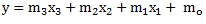
However, there might be occasion to obtain a better fit using the natural logarithm of the independent variables, using the following equation.
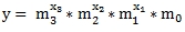
The XLeratorDB GROWTHMX and LOGEST functions are designed with this second equation in mind. Let's look at how that works based upon the following data.
|
x1
|
x2
|
x3
|
y
|
|
12
|
22
|
29
|
3.63
|
|
23
|
3
|
49
|
10.11
|
|
33
|
48
|
16
|
27.26
|
|
30
|
13
|
31
|
20.45
|
|
13
|
18
|
15
|
3.71
|
|
47
|
30
|
29
|
110.83
|
|
32
|
34
|
5
|
24.89
|
|
1
|
14
|
6
|
1.26
|
|
21
|
43
|
10
|
8.39
|
Let’s put this data into a table. I will add an identity column to keep track of the rows.
SELECT IDENTITY(int,1,1) as rn
,*
INTO #L
FROM (VALUES (12,22,29,3.63)
,(23,3,49,10.11)
,(33,48,16,27.26)
,(30,13,31,20.45)
,(13,18,15,3.71)
,(47,30,29,110.83)
,(32,34,5,24.89)
,(1,14,6,1.26)
,(21,43,10,8.39)
)n(x1,x2,x3,y)
Using this data, we can come up with a predicted y-value for any combination of independent variables using the XLeratorDB GROWTHMX function. Let's see what happens when x1 = 5, x2 = 10, and x3 = 15.
SELECT wct.GROWTHMX('#L','y,x1,x2,x3','',NULL,1,'5,10,15','True') as [Predicted Value]
This produces the following result.
Predicted Value
----------------------
1.79113665749749
Let's compare the GROWTHMX result (which uses logarithmic regression) and the TRENDMX result (which use linear regression).SELECT wct.GROWTHMX('#L','y,x1,x2,x3','',NULL,1,'5,10,15','True') as [Growth Predicted Value]
,wct.TRENDMX('#L','y,x1,x2,x3','',NULL,1,'5,10,15','True') as [Trend Predicted Value]
This produces the following result.
Growth Predicted Value Trend Predicted Value
---------------------- ----------------------
1.79113665749749 -9.90402086138496
Which of these predicted values is the better estimate?
The best way to answer that question is to look at the R2. The R2 values is always between 0 and 1, with an R2 of 1 representing a perfect correlation in the sample and an R2 of 0 indicating that the regression equation is not helpful in determining the predicted value. We can get R2 from the LINEST and LOGEST functions.
SELECT a.stat_val as [Logarithmic r-squared]
,b.stat_val as [Linear r-squared]
FROM wct.LOGEST('#L','y,x1,x2,x3','',NULL,1,'TRUE') a
,wct.LINEST('#L','y,x1,x2,x3','',NULL,1,'TRUE') b
WHERE a.stat_name = 'rsq'
AND b.stat_name = 'rsq'
This produces the following result.
Logarithmic r-squared Linear r-squared
---------------------- ----------------------
0.999554565264529 0.683715426076981
As we can plainly see, the logarithmic R2 is pretty close to 1 while the linear R2 is about .684 indicating that logarithmic regression is actually a much better predictor than linear regression.
As we did in the linear regression article, let’s calculate the predicted for each row in the #L temp table and compare it to the actual assessed value using the GROWTHMX function instead of the TRENDMX function.
SELECT rn
,y
,wct.GROWTHMX('#L','y,x1,x2,x3','',NULL,1,'SELECT x1,x2,x3 FROM #L WHERE rn = ' + cast(rn as varchar(max)),'True') as [Predicted Value]
FROM #L
The results look like this.
|
rn
|
y
|
Predicted Value
|
|
1
|
3.63
|
3.522199
|
|
2
|
10.11
|
10.28974
|
|
3
|
27.26
|
27.40381
|
|
4
|
20.45
|
20.48777
|
|
5
|
3.71
|
3.907865
|
|
6
|
110.83
|
107.5953
|
|
7
|
24.89
|
25.03458
|
|
8
|
1.26
|
1.214487
|
|
9
|
8.39
|
8.508941
|
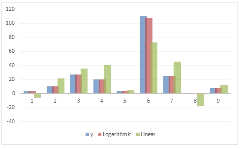
For illustrative purposes I graphed the results of the following SQL statement, to provide a visualization contrasting the goodness of fit between the logarithmic and linear regression.
SELECT rn
,y
,wct.GROWTHMX('#L','y,x1,x2,x3','',NULL,1,'SELECT x1,x2,x3 FROM #L WHERE rn = ' + cast(rn as varchar(max)),'True') as [Logarithmic]
,wct.TRENDMX('#L','y,x1,x2,x3','',NULL,1,'SELECT x1,x2,x3 FROM #L WHERE rn = ' + cast(rn as varchar(max)),'True') as [Linear]
FROM #L
As with TRENDMX, the GROWTHMX function can be computationally intensive. For every row in the resultant table, the function executed dynamic SQL which returning the specified columns of the #L table. That data are then used in an ordinary least square calculation which returns the coefficients which are then used with the new x-values to calculate the predicted value.Even though that calculation is done 9 times, the coefficients are the same for each row. This is true because the data are not dynamic—we are using the same data each time.
If we returned 100 rows then the calculation would be done 100 times; 1,000 rows, 1,000 times. For a small table like the one that we are dealing with here, the overhead isn’t too great, but if we were dealing with 25 variables, or 50 variables, or even 100 then we could be talking about considerable amounts of processing time.[1]
In situations like this, where we want to calculate many predicted values using the same coefficients, it is quite easy to use the LOGEST function to calculate the coefficient once and then apply the coefficients once to the new x-values and achieve stunning increases in performance.
The following SQL will store the coefficients in a table called #coef.
SELECT idx, stat_val as m
INTO #coef
FROM wct.LOGEST('#L','y,x1,x2,x3','',NULL,1,'TRUE')
WHERE stat_name = 'm'
The #coef table contains the following values.
|
idx
|
m
|
|
0
|
1.107411
|
|
1
|
1.102683
|
|
2
|
0.999771
|
|
3
|
0.999625
|
Both the Excel LINEST and LOGEST function return the m-values in the opposite order of the new x-values. In other words, Excel returns the m-values as a vector in the following order:
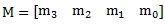
whereas the x-values are passed into the function in this order.
The XLeratorDB LOGEST function returns the coefficients in 3rd normal form eliminating any concern as to how they are physically stored. We just need to join the appropriate x-values to the appropriate m-values and perform the model calculation, which is quite simple.
But, first we have to take our x-values, which are stored in columns x1, x2, x3 and turn them into rows. We will store the normalized new x-values in a temp table called #newx. We will use the x1, x2, and x3 values from the #L table to populate the #newx table.
SELECT #L.rn
,n.idx
,n.x
INTO #newx
FROM #L
CROSS APPLY(VALUES (0,1),(1,x1),(2,x2),(3,x3),(4,x4))n(idx,x)
Now that we have all of our data in the proper form, the calculation of the predicted values using the coefficients can be achieved using the following SQL.
SELECT rn
,WCT.PRODUCT(POWER(a.m,b.x)) as y_hat
FROM #newx b
JOIN #coef a
ON b.idx = a.idx
GROUP BY rn
ORDER BY 1
The results look like this.
|
rn
|
y_hat
|
|
1
|
3.522199
|
|
2
|
10.28974
|
|
3
|
27.40381
|
|
4
|
20.48777
|
|
5
|
3.907865
|
|
6
|
107.5953
|
|
7
|
25.03458
|
|
8
|
1.214487
|
|
9
|
8.508941
|
Which are the same as the results returned from the GROWTHMX function.
Notice that we used the XLeratorDB PRODUCT function to calculate y_hat. Since POWER(a.m,b.x) is equal to EXP(b.m * LOG(a.x)), it is possible to calculate the y-hat values without the PRODUCT function as in the following SQL.
SELECT rn
,EXP(SUM(b.x * LOG(a.m))) as y_hat
FROM #newx b
JOIN #coef a
ON b.idx = a.idx
GROUP BY rn
ORDER BY 1
What kind of performance improvements can be gained by using LOGEST instead of GROWTHMX? To answer that question, we created a table with 10 columns of x-data and 1 column with y-data. We then inserted 1,000 rows into the table, giving us 10,000 x-values and 1,000 y-values.
Using the SQL in this article, we then invoked the LOGEST function and the GROWTHMX function, using each of the 1,000 rows we had just inserted and the new x-values. In other words, we were having LOGEST calculate 1,000 predicted values and GROWTHMX calculate 1,000 predicted values. We then ran that test 100 times and average the results. This table summarizes the results.
|
Function
|
Average Time (ms)
|
|
LOGEST
|
18
|
|
GROWTHMX
|
60947
|
On average, GROWTHMX took 60,947 milliseconds (60.947 seconds) to produce 1,000 predicted values, or about 16.41/second. LOGEST, on the other hand, took 18 millisecond (.018 seconds) to produce 1,000 predicted values or 55,555 / second. In this test, using LOGEST was 3,385 times faster than using GROWTHMX. You can get a copy of the test SQL here. Your times will vary, depending upon machine configuration.

How do you decide when to use GROWTHMX and when to use LOGEST? If you are only calculating one or two predicted values, or if your source data are being updated in real time, then it makes sense to use GROWTHMX as it is less SQL and always re-calculates the coefficients using the current data. However, if you are coming up with many predictions, or your data are only updated periodically, then using LOGEST is going to give you a huge performance boost, well worth the extra SQL involved.
Multiple logarithmic regression along with multiple linear regression are extremely powerful tools for building your own predictive analytics, and by putting the calculation on the database, with the data, you can achieve some startlingly high levels of throughput for your models. XLeratorDB let's you do this, and more.
[1] This is also true in Excel and leads to long waits in re-calculating spreadsheets with complex models in them.
See Also