New SQL Server Statistical Functions in XLeratorDB/statistics 1.12
Aug
6
Written by:
Charles Flock
8/6/2013 1:50 PM

We have added new functions for calculating the statistics of inter-observer agreement, as well as enhancing existing aggregate functions which calculate descriptive statistics like variance, standard deviation, covariance, etc.
We have previously written about problems with the numerical stability of SLQ Server’s built-in aggregate functions VAR, VARP, STDEV, and STDEVP. In previous releases of XLeratorDB/statistics we have provided numerically stable two-pass solutions for these calculations. In XLeratorDB/statistics 1.12 we provide numerically stable single-pass solutions which provide greater throughput than the two-pass solutions and greater accuracy and consistency than the SQL Server built-in functions.
If you are not familiar with the problem of numerically unstable algorithms, here’s a quick example using the SQL Server built-in STDEVP function.
SELECT STDEVP(x) as [Built-in function]
FROM (VALUES
(900000016.4),
(900000010.3),
(900000018.5),
(900000006.2),
(900000010.3)
)n(x)
This produces the following result.
Built-in function
----------------------
0
If you take these 5 rows of data and put them into EXCEL, you will see that the population standard deviation is clearly not zero (provided that you are using EXCEL 2007 or greater, since EXCEL used to have exactly the same problem). Let’s compare that calculation to the calculation using the XLeratorDB STDEV_P function.
SELECT STDEVP(x) as [Built-in function]
,wct.STDEV_P(x) as [XLDB Function]
FROM (VALUES
(900000016.4),
(900000010.3),
(900000018.5),
(900000006.2),
(900000010.3)
)n(x)
This produces the following result.
Built-in function XLDB Function
---------------------- ----------------------
0 4.4822315476529
In our test environment, STDEV_P function processed about 3.8 million rows a second, but since this a single-pass aggregate function, your performance will vary depending on the number of processors as the query is automatically parallelized. This was about 4 times faster than the existing two-pass implementations on the same box. It was also faster (and more accurate) than the SQL Server built-in function.
We also added numerically stable versions of the skew, kurtosis and covariance functions and attempted to keep the names of those function consistent with EXCEL 2010. Here’s a list of those functions:
· STDEV_P —population standard deviation
· STDEV_S —sample standard deviation
· VAR_P — population variance
· VAR_S — sample variance
COVARIANCE_P and COVARIANCE_S are multi-input aggregate functions requiring different versions for SQL Server 2005 where the x- and y-values are concatenated and passed into the function as a string.
We also changed the algorithms for some existing functions to be consistent with these new functions and to avoid any potential issues with numeric instability. The changed functions are:
We have also introduced new functions that deal with a category of statistics called inter-observer agreement, also called inter-rater reliability, inter-rater agreement, or concordance. These statistics generally deal with how much agreement there is between and among raters. The new XLeratorDB functions provide capabilities for the calculation of:
· Intra-class coefficient
· Cohen’s Kappa
· Kendall’s tau
· Kendall’s w
· McNemar chi-squared test for symmetry
· Spearman’s rank correlation coefficient
· Wilcoxon matched-pair signed-rank test
We have also provided ancillary functions for the calculation of:
· RANK_AVG — Average Ranks (i.e. calculating ranks with ties)
We decided to implement these as table-valued functions rather than as aggregate functions as you want to know not just the value of the test statistic, but also the p-value and other characteristics. By using a table-valued function implementation, we gather the data once, and return multiple values with a single invocation whereas an aggregate implementation would require multiple invocations.
For example, in the calculation of Cohen’s Kappa there are 8 different columns returned by the KAPPA_COHEN_TV function:
· Pa —relative observed agreement among raters
· Pc —hypothetical probability of chance agreement
· K —test statistic (kappa)
· P —p-value
· Z — normalized kappa
· SE —standard error
· NS —number of subjects
· NR —number of ratings
To return all 8 values using aggregate functions would require 8 passes through the data; one for each return value. We looked at both approaches, and it became clear that having a table-valued function that would return 8 values was much faster than having an aggregate function which could return any of the 8 values but which would have to be invoked 8 times in a TSQL statement to achieve the same result.
The unifying theme of these analyses is that they rely on contingency tables to develop their statistics. Generally, a contingency table can be thought of as a cross-tabulation of underlying data. Packages like MATLAB and SPSS have built-in cross tab functions that can be used as the starting point for calculating some of these statistics.
TSQL is not so good with cross tabs. While there is a PIVOT function, it can be trickier than you would like to get the cross tab rendered accurately. Additionally, you are then stuck with de-normalized data, which is not going to lend itself to generic SQL to do the calculations, since you will need to know how many columns you are processing and you will also need to know the column names.
Let’s look at just one pitfall that can arise using PIVOT to create a cross tab.
First, we will put some data into a table. The data consists of ratings from 2 raters for 20 subjects. The ratings can be from 1 to 6. We want to create a cross-tab of the ratings. Since there are 2 raters, we would expect the cross tab to be a square matrix with the rows representing rater 1 ratings and the columns represent rater 2 ratings.
SELECT *
INTO #c
FROM (
SELECT 3,3 UNION ALL
SELECT 3,6 UNION ALL
SELECT 3,4 UNION ALL
SELECT 4,6 UNION ALL
SELECT 5,2 UNION ALL
SELECT 5,4 UNION ALL
SELECT 2,2 UNION ALL
SELECT 3,4 UNION ALL
SELECT 5,3 UNION ALL
SELECT 2,3 UNION ALL
SELECT 2,2 UNION ALL
SELECT 6,3 UNION ALL
SELECT 1,3 UNION ALL
SELECT 5,3 UNION ALL
SELECT 2,2 UNION ALL
SELECT 2,2 UNION ALL
SELECT 1,1 UNION ALL
SELECT 2,3 UNION ALL
SELECT 4,3 UNION ALL
SELECT 3,4
)n(r1, r2)
Next we can create the cross-tab using the PIVOT function.
SELECT r2,[1],[2],[3],[4],[5],[6]
FROM (
SELECT r2, r1, COUNT(*) as N
FROM #c
GROUP BY r2, r1
) d
PIVOT(sum(N) for r1 in([1],[2],[3],[4],[5],[6]))as P
This produces the following result.
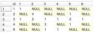
Right away we can see that the number of rows and the number of columns are not equal, therefore the cross-tab is not square. If we want to make this cross-tab square, we can change the SQL.
SELECT r1,[1],[2],[3],[4],[5],[6]
FROM (
SELECT r2, r1, COUNT(*) as N
FROM #c
GROUP BY r2, r1
) d
PIVOT(sum(N) for r2 in([1],[2],[3],[4],[5],[6]))as P
This produces the following result.
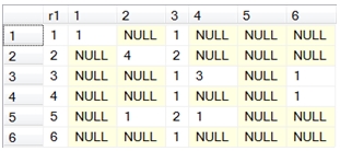
Now we have a contingency table.
The contingency table then can be used to calculate column totals, row totals, expected values, and may have weights applied to it in those calculations. I should also point out that it is not strictly necessary to use a contingency to calculate the row and column totals; this can be done in TSQL without too much effort, though the complexity increases dramatically when weightings are applied and can become insanely complex when trying to calculate the standard error and the p-value.
With the introduction of these new functions, you don’t have to worry about that complexity, at all. For example, if you wanted to calculate Cohen’s kappa based on the data in the example, you can simply enter the following SQL.
SELECT *
FROM wct.KAPPA_COHEN_TV('SELECT r2,r1 FROM #c', NULL)
This produces the following result.

The list of new table-valued functions is:
· ICC_TV —Intra-class coefficient
· WMPSR_TV —Wilcoxon matched-pair signed-rank test
We have also added scalar implementations of these functions, in case you only want one value returned, as it makes the SQL somewhat simpler. The scalar functions have the same name as the table-valued functions without the _TV at the end.
Finally, we have the scalar function PSIGNRANK which lets you calculate the Wilcoxon distribution independently of any inter-observer agreement calculation.
We think that these functions are a perfect example of the type of in-database analytics that you can do in SQL Server, eliminating the need to drag the data across the network into another platform for analysis. With XLeratorDB you can analyze the data where it is stored and even persist the results to the database without having to anything more than T-SQL. Let us know what you think.