Calculating the beta of a stock or portfolio in SQL Server
Jan
23
Written by:
Charles Flock
1/23/2013 11:57 AM

In this article we look at how moving a traditional spreadsheet calculation into SQL Server simplifies the calculation while also allowing you to analyze more data in more different ways than you would think possible
The formula for calculating the beta of a stock or portfolio is:

Where ra is the return of the asset and rb is the return of the portfolio benchmark. Substituting some of the terms, gives us the following equation:

Of course, n cancels out in the numerator and denominator, leaving us with the following equation:

which just happens to be the definition of the SLOPE function. Thus the beta of a stock or portfolio is the SLOPE of the asset returns and the benchmark returns. Let’s look at an example.
SELECT wct.COVAR(Ra, Rb) / VARP(Rb) as Beta
,wct.SLOPE(Ra, Rb) as Slope
FROM (VALUES
('2013-01-02',-0.060451,0.041923),
('2012-12-03',-0.090743,0.007068),
('2012-11-01',-0.012369,0.002847),
('2012-10-01',-0.107609,-0.019789),
('2012-09-04',0.002794,0.024236),
('2012-08-01',0.093891,0.019763),
('2012-07-02',0.045814,0.012598),
('2012-06-01',0.010862,0.039555),
('2012-05-01',-0.010711,-0.062651),
('2012-04-02',-0.025965,-0.007497),
('2012-03-01',0.105269,0.031332),
('2012-02-01',0.188326,0.040589),
('2012-01-03',0.127092,0.043583),
('2011-12-01',0.059656,0.008533),
('2011-11-01',-0.05578,-0.005059),
('2011-10-03',0.061541,0.107723),
('2011-09-01',-0.009123,-0.071762),
('2011-08-01',-0.014469,-0.056791),
('2011-07-01',0.16326,-0.021474),
('2011-06-01',-0.034951,-0.018258),
('2011-05-02',-0.00657,-0.013501),
('2011-04-01',0.004661,0.028495),
('2011-03-01',-0.01331,-0.001047),
('2011-02-01',0.040942,0.031957),
('2011-01-03',0.051952,0.022646),
('2010-12-01',0.036672,0.0653),
('2010-11-01',0.033788,-0.00229),
('2010-10-01',0.060729,0.036856),
('2010-09-01',0.167206,0.087551),
('2010-08-02',-0.055022,-0.047449),
('2010-07-01',0.022742,0.068778),
('2010-06-01',-0.020815,-0.053882),
('2010-05-03',-0.016113,-0.081976),
('2010-04-01',0.11102,0.014759),
('2010-03-01',0.148457,0.058796),
('2010-02-01',0.065399,0.028514),
('2010-01-04',-0.088615,-0.036974),
('2009-12-01',0.054151,0.017771),
('2009-11-02',0.060533,0.057364),
('2009-10-01',0.016982,-0.019762),
('2009-09-01',0.101901,0.035723),
('2009-08-03',0.029515,0.03356),
('2009-07-01',0.147117,0.074142),
('2009-06-01',0.048808,0.000196),
('2009-05-01',0.079298,0.053081),
('2009-04-01',0.197044,0.093925),
('2009-03-02',0.177022,0.085405),
('2009-02-02',-0.009178,-0.109931),
('2009-01-02',0.056028,-0.085657)
)n(tDate, Ra, Rb)
This produces the following result.
Beta Slope
---------------------- ----------------------
0.86600592673868 0.86600592673868
As you can see the Beta and the SLOPE are the same.
Interpreting the Beta value is beyond the scope of this article, as we are concerned with the mechanics of the beta calculation, especially for many assets and benchmarks at the same time. However, it is very important to note that Beta is a measure that compares returns not prices. This leaves us with the not-so-small task of calculating the returns. The math for the return calculation is straightforward enough.

Where Pt is the price (or value) of the asset at time t.
If you are a SQL Server 2008 user, you can use the XLeratorDB LAG function to do this calculation. SQL Server 2012 users can use the LAG function in SQL Server 2012. Here’s an example, using the price data to calculate the return values used in the previous example.
SELECT tDate
,ROUND(Pa / wct.LAG(Pa,1,NULL,ROW_NUMBER() OVER (ORDER BY tDate),0) - 1, 6) as Ra
,ROUND(Pb / wct.LAG(Pb,1,NULL,ROW_NUMBER() OVER (ORDER BY tDate),1) - 1, 6) as Rb
FROM (VALUES
('2013-01-02',500,1485.98),
('2012-12-03',532.17,1426.19),
('2012-11-01',585.28,1416.18),
('2012-10-01',592.61,1412.16),
('2012-09-04',664.07,1440.67),
('2012-08-01',662.22,1406.58),
('2012-07-02',605.38,1379.32),
('2012-06-01',578.86,1362.16),
('2012-05-01',572.64,1310.33),
('2012-04-02',578.84,1397.91),
('2012-03-01',594.27,1408.47),
('2012-02-01',537.67,1365.68),
('2012-01-03',452.46,1312.41),
('2011-12-01',401.44,1257.6),
('2011-11-01',378.84,1246.96),
('2011-10-03',401.22,1253.3),
('2011-09-01',377.96,1131.42),
('2011-08-01',381.44,1218.89),
('2011-07-01',387.04,1292.28),
('2011-06-01',332.72,1320.64),
('2011-05-02',344.77,1345.2),
('2011-04-01',347.05,1363.61),
('2011-03-01',345.44,1325.83),
('2011-02-01',350.1,1327.22),
('2011-01-03',336.33,1286.12),
('2010-12-01',319.72,1257.64),
('2010-11-01',308.41,1180.55),
('2010-10-01',298.33,1183.26),
('2010-09-01',281.25,1141.2),
('2010-08-02',240.96,1049.33),
('2010-07-01',254.99,1101.6),
('2010-06-01',249.32,1030.71),
('2010-05-03',254.62,1089.41),
('2010-04-01',258.79,1186.69),
('2010-03-01',232.93,1169.43),
('2010-02-01',202.82,1104.49),
('2010-01-04',190.37,1073.87),
('2009-12-01',208.88,1115.1),
('2009-11-02',198.15,1095.63),
('2009-10-01',186.84,1036.19),
('2009-09-01',183.72,1057.08),
('2009-08-03',166.73,1020.62),
('2009-07-01',161.95,987.48),
('2009-06-01',141.18,919.32),
('2009-05-01',134.61,919.14),
('2009-04-01',124.72,872.81),
('2009-03-02',104.19,797.87),
('2009-02-02',88.52,735.09),
('2009-01-02',89.34,825.88),
('2008-12-08',84.6,903.25)
)n(tDate, Pa, Pb)
This produces the following result.
tDate Ra Rb
---------- ---------------------- ----------------------
2008-12-08 NULL NULL
2009-01-02 0.056028 -0.085657
2009-02-02 -0.009178 -0.109931
2009-03-02 0.177022 0.085405
2009-04-01 0.197044 0.093925
2009-05-01 0.079298 0.053081
2009-06-01 0.048808 0.000196
2009-07-01 0.147117 0.074142
2009-08-03 0.029515 0.03356
2009-09-01 0.101901 0.035723
2009-10-01 0.016982 -0.019762
2009-11-02 0.060533 0.057364
2009-12-01 0.054151 0.017771
2010-01-04 -0.088615 -0.036974
2010-02-01 0.065399 0.028514
2010-03-01 0.148457 0.058796
2010-04-01 0.11102 0.014759
2010-05-03 -0.016113 -0.081976
2010-06-01 -0.020815 -0.053882
2010-07-01 0.022742 0.068778
2010-08-02 -0.055022 -0.047449
2010-09-01 0.167206 0.087551
2010-10-01 0.060729 0.036856
2010-11-01 0.033788 -0.00229
2010-12-01 0.036672 0.0653
2011-01-03 0.051952 0.022646
2011-02-01 0.040942 0.031957
2011-03-01 -0.01331 -0.001047
2011-04-01 0.004661 0.028495
2011-05-02 -0.00657 -0.013501
2011-06-01 -0.034951 -0.018258
2011-07-01 0.16326 -0.021474
2011-08-01 -0.014469 -0.056791
2011-09-01 -0.009123 -0.071762
2011-10-03 0.061541 0.107723
2011-11-01 -0.05578 -0.005059
2011-12-01 0.059656 0.008533
2012-01-03 0.127092 0.043583
2012-02-01 0.188326 0.040589
2012-03-01 0.105269 0.031332
2012-04-02 -0.025965 -0.007497
2012-05-01 -0.010711 -0.062651
2012-06-01 0.010862 0.039555
2012-07-02 0.045814 0.012598
2012-08-01 0.093891 0.019763
2012-09-04 0.002794 0.024236
2012-10-01 -0.107609 -0.019789
2012-11-01 -0.012369 0.002847
2012-12-03 -0.090743 0.007068
2013-01-02 -0.060451 0.041923
It would seem straightforward, then, that we could change our SELECT statement slightly and use the SLOPE function to calculate the beta directly from the price data. But, when we do that, we generate an error message.
SELECT wct.SLOPE(
ROUND(Pa / wct.LAG(Pa,1,NULL,ROW_NUMBER() OVER (ORDER BY tDate),0) - 1, 6)
,ROUND(Pb / wct.LAG(Pb,1,NULL,ROW_NUMBER() OVER (ORDER BY tDate),1) - 1, 6)
)
This produces the following error message.
.Net SqlClient Data Provider: Msg 4109, Level 15, State 1, Line 2
Windowed functions cannot be used in the context of another windowed function or aggregate.
We get the same message in SQL Server 2012 using the built-in LAG function.
SELECT wct.SLOPE(
ROUND(Pa / LAG(Pa) OVER (ORDER BY tDate) - 1, 6)
,ROUND(Pb / LAG(Pb) OVER (ORDER BY tDate) - 1, 6)
)
This produces the following result.
Msg 4109, Level 15, State 1, Line 2
Windowed functions cannot be used in the context of another windowed function or aggregate.
Faced with this limitation, we implemented the EQBETA function, which will calculate the beta from the price data.[1] The EQBETA function makes things really simple, taking in the price data, converting it to return data, and then calculating the SLOPE. This makes the SQL very simple and straightforward.
SELECT wct.EQBETA(tdate, Pa, Pb) as Beta
FROM (VALUES
('2013-01-02',500,1485.98),
('2012-12-03',532.17,1426.19),
('2012-11-01',585.28,1416.18),
('2012-10-01',592.61,1412.16),
('2012-09-04',664.07,1440.67),
('2012-08-01',662.22,1406.58),
('2012-07-02',605.38,1379.32),
('2012-06-01',578.86,1362.16),
('2012-05-01',572.64,1310.33),
('2012-04-02',578.84,1397.91),
('2012-03-01',594.27,1408.47),
('2012-02-01',537.67,1365.68),
('2012-01-03',452.46,1312.41),
('2011-12-01',401.44,1257.6),
('2011-11-01',378.84,1246.96),
('2011-10-03',401.22,1253.3),
('2011-09-01',377.96,1131.42),
('2011-08-01',381.44,1218.89),
('2011-07-01',387.04,1292.28),
('2011-06-01',332.72,1320.64),
('2011-05-02',344.77,1345.2),
('2011-04-01',347.05,1363.61),
('2011-03-01',345.44,1325.83),
('2011-02-01',350.1,1327.22),
('2011-01-03',336.33,1286.12),
('2010-12-01',319.72,1257.64),
('2010-11-01',308.41,1180.55),
('2010-10-01',298.33,1183.26),
('2010-09-01',281.25,1141.2),
('2010-08-02',240.96,1049.33),
('2010-07-01',254.99,1101.6),
('2010-06-01',249.32,1030.71),
('2010-05-03',254.62,1089.41),
('2010-04-01',258.79,1186.69),
('2010-03-01',232.93,1169.43),
('2010-02-01',202.82,1104.49),
('2010-01-04',190.37,1073.87),
('2009-12-01',208.88,1115.1),
('2009-11-02',198.15,1095.63),
('2009-10-01',186.84,1036.19),
('2009-09-01',183.72,1057.08),
('2009-08-03',166.73,1020.62),
('2009-07-01',161.95,987.48),
('2009-06-01',141.18,919.32),
('2009-05-01',134.61,919.14),
('2009-04-01',124.72,872.81),
('2009-03-02',104.19,797.87),
('2009-02-02',88.52,735.09),
('2009-01-02',89.34,825.88),
('2008-12-08',84.6,903.25)
)n(tDate, Pa, Pb)
This produces the following result.
Beta
----------------------
0.866005982032534
Having the EQBETA function lets us do some interesting things. We have created a very simple table called eqprices, which contains a ticker, a date, and a price. Then we randomly generated 1.637 million rows of data. Part of the data is the indexes against which we want to benchmark, which have tickers of SPX, COMP, and DJIA. The key to the table is ticker and date. In this statement, we calculate the beta for all 500 tickers using prices from 2012-Jan-01 onward.
SELECT e1.ticker
,wct.EQBETA(e1.tdate,e2.price_closing,e1.price_closing) as beta
FROM eqprices e1
JOIN eqprices e2
ON e2.ticker = 'SPX'
AND e1.ticker <> 'SPX'
AND e1.tdate = e2.tdate
AND e1.tdate > '2012-01-01'
GROUP BY e1.ticker
ORDER BY 1
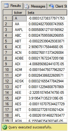
Here are are the first few rows returned by the SELECT.

And here are the statistics generated by the statement.
As you can see, the total execution time was 1242 milliseconds; a little more than a second. And very little data moved back and forth; all the calculations are done on the database. If you’re interested, I did this in SQL Server 2008 R2 with the following machine:

Essentially, this makes the calculation of beta a trivial exercise. In this example we will compare the 1-year and 3-year betas.
SELECT *
FROM (
SELECT e1.ticker
,1 AS yr
,wct.EQBETA(e1.tdate,e2.price_closing,e1.price_closing) as [BETA]
FROM eqprices e1
JOIN eqprices e2
ON e2.ticker = 'COMP'
AND e1.ticker <> 'COMP'
AND e1.tdate = e2.tdate
AND e1.tdate > DATEADD(yy,-1,'2012-12-10')
GROUP BY e1.ticker
UNION ALL
SELECT e1.ticker
,3
,wct.EQBETA(e1.tdate,e2.price_closing,e1.price_closing) as [BETA]
FROM eqprices e1
JOIN eqprices e2
ON e2.ticker = 'COMP'
AND e1.ticker <> 'COMP'
AND e1.tdate = e2.tdate
AND e1.tdate > DATEADD(yy,-3,'2012-12-10')
GROUP BY e1.ticker
) d
PIVOT(SUM(BETA) FOR YR in([1],[3])) p
Here are the first few rows returned by the statement.
Ticker 1 3
------ ---------------------- ----------------------
AAPL 0.000528774432742821 0.000215904529669967
ABC 0.000182397495347866 -3.24081991621297E-05
ABT -0.000181830782491652 -0.000237210203976776
ACN 0.000340978117436343 -8.0011175435327E-05
ADI 2.28440291047768E-05 -0.000126471901695446
ADP 0.000229319494989254 -0.000208379877589705
ADSK 0.000332881423336462 0.000122985748424428
AEE -5.43281821282431E-05 -1.87492484463807E-05
AET 0.000318655916427984 -0.000467593446370447
AIV -1.07136028956299E-05 -0.000176516458497995
ALL 0.000173155734607894 5.42232046111245E-05
AMD 4.11487375122197E-05 -6.38008640377941E-05
AMGN -0.000511500572982186 -8.55573771463149E-06
AMT 5.26011740458716E-05 -8.7465886377795E-05
AMZN -0.000375288599107781 -0.000415651363119432
AN -0.000149609906378837 -0.000187809955072543
AON -0.000373286712898433 -0.000306074496281714
APH -4.71289519772561E-05 -8.76167743634843E-05
ATI 0.000366154256857682 0.000268443744337173
AVB -0.00021712719685472 0.000242470277203392
AVP 0.000145701364842811 -0.000145276357886447
AVY -0.000125384582922887 8.78985919606747E-05
AXP 0.000227156771000262 0.000175801041161843
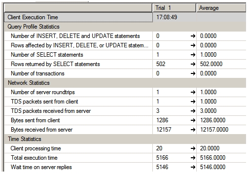
Here are the client statistics.

Again, very little data moving around and a response of just a little over 5 second (5,166 milliseconds).
There is one other very interesting aspect of implementing the EQBETA function in SQL Server. Let’s assume that you want to evaluate multiple portfolios against the S&P 500. We will keep this example simple, with 5 portfolios having valuations for the last 12 months. We put the closing prices for three benchmarks in a separate table.
SELECT *
INTO #p
FROM (VALUES
('A','2012-12-31',1619488.45), ('B','2012-12-31',1733551.06), ('C','2012-12-31',1139347.79), ('D','2012-12-31',1220850.78), ('E','2012-12-31',1709084.06), ('A','2012-11-30',1548974.65), ('B','2012-11-30',1652066.38), ('C','2012-11-30',1092770.75), ('D','2012-11-30',1169707.78), ('E','2012-11-30',1653648.97),
('A','2012-10-31',1534294.05), ('B','2012-10-31',1645536.38), ('C','2012-10-31',1087152.01), ('D','2012-10-31',1157360.70), ('E','2012-10-31',1641716.47), ('A','2012-09-30',1530396.59), ('B','2012-09-30',1652565.23), ('C','2012-09-30',1087645.04), ('D','2012-09-30',1145962.15), ('E','2012-09-30',1643447.51),
('A','2012-08-31',1553843.15), ('B','2012-08-31',1701551.89), ('C','2012-08-31',1116895.87), ('D','2012-08-31',1163873.47), ('E','2012-08-31',1669982.53), ('A','2012-07-31',1515595.45), ('B','2012-07-31',1650972.55), ('C','2012-07-31',1100567.75), ('D','2012-07-31',1126653.25), ('E','2012-07-31',1625546.45),
('A','2012-06-30',1498418.53), ('B','2012-06-30',1633876.71), ('C','2012-06-30',1072507.35), ('D','2012-06-30',1108187.13), ('E','2012-06-30',1592793.26), ('A','2012-05-31',1482852.09), ('B','2012-05-31',1621556.70), ('C','2012-05-31',1063470.37), ('D','2012-05-31',1102128.03), ('E','2012-05-31',1588032.91),
('A','2012-04-30',1431248.54), ('B','2012-04-30',1567243.99), ('C','2012-04-30',1024483.72), ('D','2012-04-30',1057750.20), ('E','2012-04-30',1516087.12), ('A','2012-03-31',1527399.35), ('B','2012-03-31',1663124.21), ('C','2012-03-31',1093775.11), ('D','2012-03-31',1118780.43), ('E','2012-03-31',1631518.12),
('A','2012-02-29',1541733.61), ('B','2012-02-29',1686221.23), ('C','2012-02-29',1110428.76), ('D','2012-02-29',1122144.05), ('E','2012-02-29',1656863.99), ('A','2012-01-31',1481677.70), ('B','2012-01-31',1631354.88), ('C','2012-01-31',1078261.65), ('D','2012-01-31',1081029.91), ('E','2012-01-31',1592935.70),
('A','2011-12-31',1433249.00), ('B','2011-12-31',1563365.00), ('C','2011-12-31',1045243.00), ('D','2011-12-31',1034093.00), ('E','2011-12-31',1545505.00)
)n(port,tDate,val)
SELECT *
INTO #b
FROM (VALUES
('SPX','2012-12-31',1485.98),
('SPX','2012-11-30',1426.19),
('SPX','2012-10-31',1416.18),
('SPX','2012-09-30',1412.16),
('SPX','2012-08-31',1440.67),
('SPX','2012-07-31',1406.58),
('SPX','2012-06-30',1379.32),
('SPX','2012-05-31',1362.16),
('SPX','2012-04-30',1310.33),
('SPX','2012-03-31',1397.91),
('SPX','2012-02-29',1408.47),
('SPX','2012-01-31',1365.68),
('SPX','2011-12-31',1312.41),
('COMP','2012-12-31',3091.33),
('COMP','2012-11-30',3029.21),
('COMP','2012-10-31',2987.54),
('COMP','2012-09-30',3130.31),
('COMP','2012-08-31',3063.25),
('COMP','2012-07-31',2956.72),
('COMP','2012-06-30',2938.41),
('COMP','2012-05-31',2810.13),
('COMP','2012-04-30',3044.79),
('COMP','2012-03-31',3085.94),
('COMP','2012-02-29',2979.11),
('COMP','2012-01-31',2830.10),
('COMP','2011-12-31',2657.39),
('DJIA','2012-12-31',13104.3),
('DJIA','2012-11-30',13027.73),
('DJIA','2012-10-31',13099.19),
('DJIA','2012-09-30',13437.66),
('DJIA','2012-08-31',13092.15),
('DJIA','2012-07-31',13007.47),
('DJIA','2012-06-30',12879.71),
('DJIA','2012-05-31',12391.56),
('DJIA','2012-04-30',13214.16),
('DJIA','2012-03-31',13211.36),
('DJIA','2012-02-29',12952.29),
('DJIA','2012-01-31',12632.76),
('DJIA','2011-12-31',12221.19)
)m(ticker,tDate,pr)
The calculation of the beta for each of the portfolios is straightforward. We will use SPX as the benchmark.
SELECT #p.port
,wct.EQBETA(#p.tDate,#p.val,#b.pr) as Beta
FROM #p
JOIN #b
ON #b.tDate = #p.tDate
AND #b.ticker = 'SPX'
GROUP BY #p.port
ORDER BY 1
This produces the following result.
port Beta
---- ----------------------
A 0.983910724951417
B 1.03034658060587
C 1.002214561704
D 0.960458214873104
E 1.05265687457901
What if we wanted to calculate the beta across all portfolios? This is extremely easy using the EQBETA function.
SELECT wct.EQBETA(#p.tDate,#p.val,#b.pr) as Beta
FROM #p
JOIN #b
ON #b.tDate = #p.tDate
AND #b.ticker = 'SPX'
This produces the following result.
Beta
----------------------
1.0095843955307
In this example, we calculate the beta for each portfolio against different benchmarks.
SELECT #p.port
,#b.ticker
,wct.EQBETA(#p.tDate,#p.val,#b.pr) as Beta
FROM #p
JOIN #b
ON #b.tDate = #p.tDate
GROUP BY #p.port
,#b.ticker
ORDER BY 2,1
This produces the following result.
port ticker Beta
---- ------ ----------------------
A COMP 0.128316121199841
B COMP 0.152866971810549
C COMP 0.0658973826059795
D COMP 0.0967770193579477
E COMP 0.0607068953214639
A DJIA -0.0724662101118738
B DJIA -0.0677773954868839
C DJIA -0.1382399115682
D DJIA -0.1290499027521
E DJIA -0.187291358877354
A SPX 0.983910724951417
B SPX 1.03034658060587
C SPX 1.002214561704
D SPX 0.960458214873104
E SPX 1.05265687457901
We can use PIVOT to look at the results side-by-side.
SELECT *
FROM (
SELECT #p.port
,#b.ticker
,wct.EQBETA(#p.tDate,#p.val,#b.pr) as Beta
FROM #p
JOIN #b
ON #b.tDate = #p.tDate
GROUP BY #p.port
,#b.ticker
) d
PIVOT(SUM(BETA) FOR ticker in(COMP,DJIA,SPX)) p
This produces the following result.
port COMP DJIA SPX
---- ---------------------- ---------------------- ----------------------
A 0.128316121199841 -0.0724662101118738 0.983910724951417
B 0.152866971810549 -0.0677773954868839 1.03034658060587
C 0.0658973826059795 -0.1382399115682 1.002214561704
D 0.0967770193579477 -0.1290499027521 0.960458214873104
E 0.0607068953214639 -0.187291358877354 1.05265687457901
Finally, we can look at all portfolios against each of the benchmarks.
SELECT #b.ticker
,wct.EQBETA(#p.tDate,#p.val,#b.pr) as Beta
FROM #p
JOIN #b
ON #b.tDate = #p.tDate
GROUP BY #b.ticker
ORDER BY 1
This produces the following result.
ticker Beta
------ ----------------------
COMP 0.103462228945628
DJIA -0.117485238733587
SPX 1.0095843955307
The EQBETA function can be an important tool in equity analysis, along with the hundreds of other financial, statistical, and mathematical functions in XLeratorDB. If you are interested in trying this out for yourself, download the 15-day free trial today and let us know what you think.
[1] Why didn’t we call this the BETA function? We already have a BETA function which calculates Γ(a)Γ(b)/Γ(a+b).