Creating a Bond Amortization Schedule in SQL Server
Apr
5
Written by:
Charles Flock
4/5/2012 8:55 PM

A look at different techniques for generating schedules to account for the premium or discount associated with the issuance or purchase of a bond using the XLeratorDB functions COUPDAYSNC, COUPNUM, DAYS360, EDATE, IRR, PRICE, PV, RATE, SeriesDate, SeriesInt, XIRR, and YIELD.
The preferred treatment to account for the interest expense associated with the issuance of a bond is to use a technique called the constant yield method also known as the effective interest method. The effective interest method is very simple in concept: the interest expense should reflect the yield on the bond. Additionally, at least in the US, the costs of issuing the bond should not be expensed as they are incurred, but rather, included as an adjustment to the cost basis for the bond and recognized over the life of the bond as part of the interest expense.
The effective interest method may also be applied to bonds that have been purchased.
The following example shows a calculation of the coupon interest payments and associated amortization of a bond issued on 15-Oct-2011 having a maturity date of 15-Oct-2013, with a 5% interest and semi-annual coupon payments. The redemption value of the bond is 100 and accrued interest is calculated on an actual/actual basis. The bond is issued at a price of 105, and this example shows the amortization of the premium of 5, using the effective interest method, as at each of the coupon dates.
/*Amortization on the Coupon Dates*/
DECLARE @s as datetime = '2011-10-15' --settlement date
DECLARE @m as datetime = '2013-10-15' --maturity date
DECLARE @rt as float = .05 --redemption
DECLARE @pr as float = 105 --price
DECLARE @rn as float = 100 --redemption
DECLARE @f as float = 2 --frequency
DECLARE @b as nvarchar(1) = 1 --basis
DECLARE @y as float =(SELECT wct.YIELD(@s,@m,@rt,@pr,@rn,@f,@b)) --yield
DECLARE @nc as float =(SELECT wct.COUPNUM(@s,@m,@f,@b)) --number of coupons
SELECT Seq as c_num --the coupon number
,convert(varchar, wct.EDATE(@m,-Seriesvalue*12/@f), 106) as c_date --the coupon date
,100 * @rt/@f as coup --the coupon amount
,wct.PRICE(wct.EDATE(@m,-Seriesvalue*12/@f),@m,@rt,@y,@rn,@f,@b) - wct.PRICE(wct.EDATE(@m,-(Seriesvalue+1)*12/@f),@m,@rt,@y,@rn,@f,@b) as amort --the amortization amount
,wct.PRICE(wct.EDATE(@m,-Seriesvalue*12/@f),@m,@rt,@y,@rn,@f,@b) as bv --the book value
FROM wct.SeriesInt(@nc-1,0,NULL,NULL,NULL)
UNION ALL
SELECT 0, convert(varchar,@s,106),0,0,@pr --the value of the bond at the start
ORDER BY 1
This produces the following result.
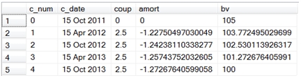
Notice that we used the XLeratorDB YIELD function to calculate the yield of the bond on the issue date. We then used the value for yield in the XLeratorDB PRICE function to calculate the book value of the bond as at the coupon date. The XLeratorDB COUPNUM function calculated the number of coupons to be paid on the bond. The SERIESINT table-valued function generated sequential numbers for each of the coupons. The EDATE function calculated the coupon dates by counting backwards from the maturity date.
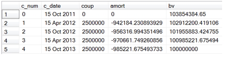
What if we wanted to record the amortization based upon the face value of the bond? Let’s change the example a little bit, and assume that face value of the issuance is USD 100 million and that the proceeds from the sale of the bond are USD 103,854,384.65. Here’s how we can generate that schedule.
/*Amortization on the Coupon Dates using face amount*/
DECLARE @s as datetime = '2011-10-15' --settlement date
DECLARE @m as datetime = '2013-10-15' --maturity date
DECLARE @rt as float = .05 --coupon rate
DECLARE @fa as float = 100000000 --face amount
DECLARE @pr as float = 103854384.65 --proceeds
DECLARE @rn as float = 100 --redemption
DECLARE @f as float = 2 --frequency
DECLARE @b as nvarchar(1) = 1 --basis
DECLARE @y as float =(SELECT wct.YIELD(@s,@m,@rt,@pr/@fa*100,@rn,@f,@b)) --yield
DECLARE @nc as float =(SELECT wct.COUPNUM(@s,@m,@f,@b)) --number of coupons
SELECT c_num
,c_date
,coup * @fa/100 as coup
,amort * @fa/100 as amort
,bv * @fa/100 as bv
--This is select from the first example put
--into a derived table
FROM (
SELECT Seq as c_num
,CAST(wct.EDATE(@m,-Seriesvalue*12/@f) as date) as c_date
,100 * @rt/@f as coup
,wct.PRICE(wct.EDATE(@m,-Seriesvalue*12/@f),@m,@rt,@y,@rn,@f,@b) - wct.PRICE(wct.EDATE(@m,-(Seriesvalue+1)*12/@f),@m,@rt,@y,@rn,@f,@b) as amort
,wct.PRICE(wct.EDATE(@m,-Seriesvalue*12/@f),@m,@rt,@y,@rn,@f,@b) as bv
FROM wct.SeriesInt(@nc-1,0,NULL,NULL,NULL)
UNION ALL
SELECT 0, @s,0,0,@pr/@fa * 100
) c
ORDER BY 1
This produces the following result.
While these examples are good at demonstrating the concept behind the effective interest method, in most accounting environments there is no link between the coupon dates on the issued bonds and the financial reporting dates, which in the US are usually at quarter end. The challenge becomes how to implement this method in such a way that we can still achieve the same treatment but fit it into the financial reporting calendar.
This is compounded by some of the conventions of the bond market with regard to the counting of dates. For purposes of this discussion we will ignore bonds that have an odd first period or an odd last period (i.e. bonds where the first and/or last period is longer or shorter than the other periods).
For most bonds, the amount of the coupons is fixed; in fact this assumption is built into the calculation of the price of the bond. When calculating the market price or the market yield of the bond on a coupon date, there is no need to know how many days there are in a coupon period; the only thing that is important is knowing the number of coupons remaining.
When performing these calculations on a date other than the coupon date, we now need to know the number of days in the coupon period as well the number of remaining coupons. This is where things get a little tricky as there are a number of ways of doing this. One way is to assume that the year is divided into 12 months of exactly 20 days (and there is actually more than one way of doing that). Another way is to assume that year is always 365 days or 360 days. Another way is to assume that year is the actual number of days in the year, either 365 or 366. These different techniques can all complicate the process of creating an amortization schedule.
In the rest of the this article, I will describe a generic approach which will work regardless of the accrual basis of the bond, and will calculate amortization amounts on a daily basis which can then be summed into whatever reporting periods make sense: monthly, quarterly, semi-anually or anually. Then I describe another tehcnique, which I will call the constant daily effective rate method, which will produce different results than the generic method, but is practiced in some juridictions.
The generic technique
This is really very simple, in that we will just calculate the yield of the bond as at its start date and then use that yield to calculate the daily change in price of the bond and record the change in price as amortization. We will set up a generic bond, and we can adjust the accrual basis to see what the effect will be. Here are the variables for our bond.
DECLARE @s as datetime = '2011-10-15' --settlement date
DECLARE @m as datetime = '2016-10-15' --maturity date
DECLARE @rt as float = .05 --coupon rate
DECLARE @fa as float = 100000000 --face amount
DECLARE @pr as float = 99275000 --proceeds
DECLARE @rn as float = 100 --redemption
DECLARE @f as float = 2 --frequency
DECLARE @b as nvarchar(1) = 0 --actual/actual basis
DECLARE @nc as float =(SELECT wct.COUPNUM(@s,@m,@f,@b)) --number of coupons
DECLARE @y as float =(SELECT wct.YIELD(@s,@m,@rt,@pr/@fa*100,@rn,@f,@b)) --yield
To generate the amortization schedule by coupon we will use the SQL from our previous example, though I have rounded the amounts to make it a little easier to read.
SELECT c_num
,c_date
,ROUND(coup * @fa/100, 2) as coup
,ROUND(amort * @fa/100, 2) as amort
,ROUND(bv * @fa/100, 2) as bv
FROM (
SELECT Seq as c_num
,convert(varchar, wct.EDATE(@m,-Seriesvalue*12/@f), 106) as c_date
,100 * @rt/@f as coup
,wct.PRICE(wct.EDATE(@m,-Seriesvalue*12/@f),@m,@rt,@y,@rn,@f,@b) - wct.PRICE(wct.EDATE(@m,-(Seriesvalue+1)*12/@f),@m,@rt,@y,@rn,@f,@b) as amort
,wct.PRICE(wct.EDATE(@m,-Seriesvalue*12/@f),@m,@rt,@y,@rn,@f,@b) as bv
FROM wct.SeriesInt(@nc-1,0,NULL,NULL,NULL)
UNION ALL
SELECT 0, convert(varchar,@s,106),0,0,@pr/@fa * 100
) c
ORDER BY 1
This produces the following result.
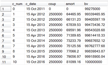
It’s pretty easy to see that in amortizing by coupon period the amortization amount increases in each succeeding period. That does not necessarily mean that it increases for each day in the period, as we will see a little later.
What would happen if we changed the interest basis from 0 to 1?
/*DECLARE @b as nvarchar(1) = 0 --basis*/
DECLARE @b as nvarchar(1) = 1 --30/360 basis
We run our SELECT statement and we discover that it produces exactly the same result. This is because the calculation of the price of a bond on the coupon dates does not factor in the number of days in the coupon period, because the number of days from the start of the coupon period to settlement date of the bond is zero.
Now we can create a daily amortization schedule, which can then be summarized into whatever periods we need. Again, I will round the amounts to make things a little easier to read.
SELECT Seq
,SeriesValue
,bv * @fa/100 as bv
,CASE NCD
WHEN 1 THEN @rt/@f * 100 - wct.BONDINT(SeriesValue,@m,@rt,100,@f,@b)
ELSE wct.BONDINT(SeriesValue+1,@m,@rt,100,@f,@b)-wct.BONDINT(SeriesValue,@m,@rt,100,@f,@b)
END * @fa/100 as [dly coup]
,([bv end] - bv) * @fa/100 as amort
,[bv end] * @fa/100 as [bv end]
FROM (
SELECT *
,wct.PRICE(SeriesValue,@m, @rt,@y,@rn,@f,@b) as bv
,wct.COUPDAYSNC(seriesvalue,@m,@f,@b) as NCD
,wct.PRICE(SeriesValue + 1,@m, @rt,@y,@rn,@f,@b) as [bv end]
from wct.SeriesDate(@s,@m-1,NULL,NULL,NULL)
) a
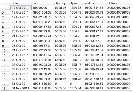
Here are the first few rows in the resultant table.
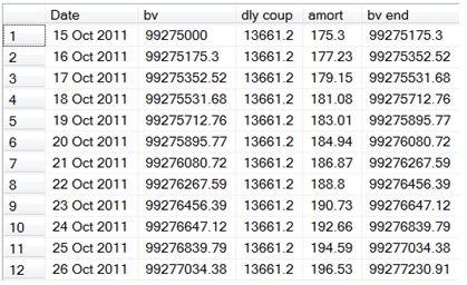
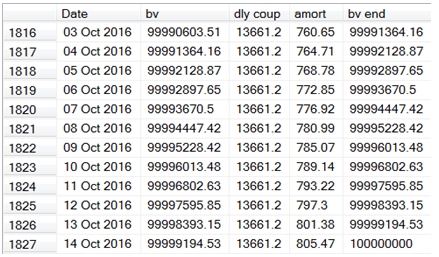
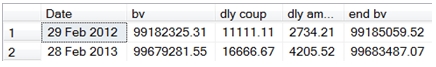
There are 1,827 rows in the resultant table, showing the beginning book value, the daily coupon, the daily amortization, and the ending book value for this bond, which has an actual/actual accrual basis (the basis code is equal to 1). We have set up this schedule to accrue on the first day and not on the last day, so that the coupon interest is fully accrued on the day before the coupon date and on the day before the maturity date. This is what the last few rows of the resultant table look like.
Let’s put this information into a temporary table so the we can analyze it a little further and hopefully make things a little less confusing.
SELECT SeriesValue as [Date]
,bv * @fa/100 as bv
,CASE NCD
WHEN 1 THEN @rt/@f * 100 - wct.BONDINT(SeriesValue,@m,@rt,100,@f,@b)
ELSE wct.BONDINT(SeriesValue+1,@m,@rt,100,@f,@b)-wct.BONDINT(SeriesValue,@m,@rt,100,@f,@b)
END * @fa/100 as [dly coup]
,([bv end] - bv) * @fa/100 as amort
,[bv end] * @fa/100 as [bv end]
INTO #am --put the results into a temp table
FROM (
SELECT *
,wct.PRICE(SeriesValue,@m, @rt,@y,@rn,@f,@b) as bv
,wct.COUPDAYSNC(seriesvalue,@m,@f,@b) as NCD
,wct.PRICE(SeriesValue + 1,@m, @rt,@y,@rn,@f,@b) as [bv end]
from wct.SeriesDate(@s,@m-1,NULL,NULL,NULL)
) a
First, let’s see how this compares to the amortization schedule we created by coupon date.
SELECT convert(varchar,CoupDate, 106) as [Coup Date]
,ROUND(MIN(bv), 2) as [Beg Book Val]
,ROUND(SUM([dly coup]), 2) as [Coup Int]
,ROUND(SUM(AMORT), 2) as Amort
,ROUND(MAX([bv end]), 2) as [End Book Val]
FROM (
SELECT *
,wct.COUPNCD(a.date,@m,@f,@b) as CoupDate
from #am a
) b
GROUP BY CoupDate
ORDER BY CoupDate
This produces the following result.
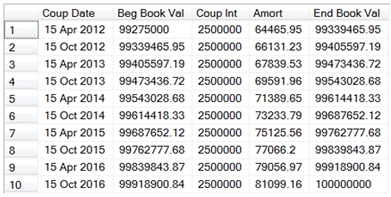
We can see that it is an exact match. And, if we changed the interest basis from 1 to any of the other supported bases (0,2,3,4), it will also match.
We could summarize the schedule into quarters (for accounting purposes) with the following SQL.
SELECT YEAR(date) as YR
,DATEPART(qq,date) as Q
,ROUND(MIN(bv), 2) as [Beg Book Val]
,ROUND(SUM([dly coup]), 2) as [Coup Int]
,ROUND(SUM(AMORT), 2) as Amort
,ROUND(MAX([bv end]), 2) as [End Book Val]
FROM #am
GROUP BY YEAR(date), DATEPART(qq,date)
ORDER BY 1,2
This produces the following result.
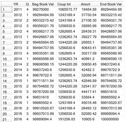
There’s a couple of things to notice here. First, unlike the schedule by coupon date, the coupon interest amount varies by quarter. This is because we have a bond with an actual/actual basis, and interest is recognized based on the actual number of days in the coupon period. The number of days in period changes from one coupon period to another, as does the number of days in the quarter from one quarter to another.
Second, notice that the amortization amount changes from quarter to quarter. In the coupon date amortization schedule, the amortization amount smoothly increased from quarter to quarter, but when we slice the same data by quarter, the amounts seem to go up and down from quarter to quarter. Also remmber that we know that the daily amortization schedule we created agrees with the coupon date amortization schedule, so we know that for each coupon period, the aggregate amounts in the daily schedule are correct.
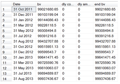
Let’s see what happens when we summarize the schedule by month.
SELECT YEAR(date) as YR
/*,DATEPART(qq,date) as Q*/
,MONTH(date) as M
,ROUND(MIN(bv), 2) as [Beg Book Val]
,ROUND(SUM([dly coup]), 2) as [Coup Int]
,ROUND(SUM(AMORT), 2) as Amort
,ROUND(MAX([bv end]), 2) as [End Book Val]
FROM #am
/*GROUP BY YEAR(date), DATEPART(qq,date)*/
GROUP BY YEAR(date), MONTH(date)
ORDER BY 1,2
Here are the first couple of dozen rows from the resultant table.
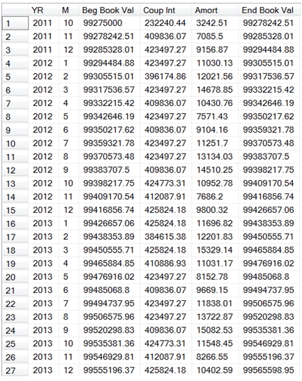
Again, we see that the amortization amount seems to increase smoothly until the month in which there is a coupon, and then the amount resets. Let’s look at the table for the month of April, 2012 and see what’s going on.
SELECT convert(varchar,Date, 106) as Date
,ROUND(bv, 2) as bv
,ROUND([dly coup], 2) as [dly coup]
,ROUND(amort, 2) as amort
,ROUND([bv end], 2) as [bv end]
FROM #am
WHERE DATE between '2012-04-01'
AND '2012-04-30'
This produces the following result.
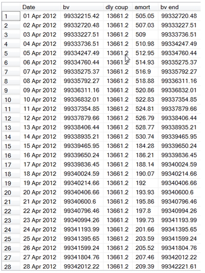
As you can see the daily amortization increases smoothly until the coupon date, 2012-04-15 and then the amount starts off much lower and increases from there. There is absolutely nothing wrong with this as the book value of the bond still correctly reflects the price of the bond holding the yield constant. As we have already demonstrated, these amounts agree with the coupon amortization schedule, and we know that the book value reflects the yield of the bond at the time it went on the balance sheet, because we are using the yield to calculate the price on each date.
The reasons for the sudden change have to do with the fact that the price of the bond changes based on the present value of the coupon payments, which are twice-yearly in this example, versus the coupon interest which is taken into income on a daily basis basically on a straight line.
The fact that the daily amortization amount goes down and could even change sign, is an artifact of the math behind bond figuration, which is far too complicated a subject to go into here.
So, while this technique is perfectly acceptable and in compliance with US accounting standards, there is an alternative method to calculating the amortization which I will call the daily effective rate.
The daily effective rate technique
Many times, institutions will create a daily amortization schedule and calculate an effective rate that they will apply to the book value from the previous day to arrive at the book value for the current day. Frequently, this effective rate is calculated using the Solver function in EXCEL. Let’s look at how we can do this in T-SQL using XLeratorDB. To do that, let’s look at some specifics, based on an actual example.
Face Value: 100,000,000
Clean Price: 99.20
Interest Rate: 7.0%
Interest Basis: Actual/365
Settle Date: 7/13/2010
Maturity Date: 10/22/2019
Effective Rate: 0.0001950076236
For purposes of this example, we will assume that interest is accrued on the last day and not on the first day, though you could certainly creat the schedule making the assumption that interest is accrued on the first day instead.
The Effective Rate was calculated by the Solver function in EXCEL and is used to create the following table (from EXCEL):
|
Date
|
Book value
|
daily coupon
|
daily effective rate
|
amortization
|
Ending book value
|
|
7/13/2010
|
99200000.00000
|
|
|
0
|
99200000.00000
|
|
7/14/2010
|
99200000.00000
|
19178.08219
|
19344.75626
|
166.6741
|
99200166.67407
|
|
7/15/2010
|
99200166.67407
|
19178.08219
|
19344.78876
|
166.7066
|
99200333.38064
|
|
7/16/2010
|
99200333.38064
|
19178.08219
|
19344.82127
|
166.7391
|
99200500.11972
|
|
7/17/2010
|
99200500.11972
|
19178.08219
|
19344.85379
|
166.7716
|
99200666.89132
|
|
7/18/2010
|
99200666.89132
|
19178.08219
|
19344.88631
|
166.8041
|
99200833.69544
|
|
7/19/2010
|
99200833.69544
|
19178.08219
|
19344.91884
|
166.8366
|
99201000.53208
|
|
7/20/2010
|
99201000.53208
|
19178.08219
|
19344.95137
|
166.8692
|
99201167.40126
|
|
7/21/2010
|
99201167.40126
|
19178.08219
|
19344.98391
|
166.9017
|
99201334.30299
|
Our starting book value is the clean price of the bond multiplied by the face amount. The daily coupon is the coupon interest rate (7.0%) divided by 365 multiplied by the face amount. The daily effective rate is the effective rate (0.0001950076236) multiplied by the book value. The amortization is the daily effective rate minus the daily coupon. The ending book value is the book value and becomes the book value for the next row in the table.
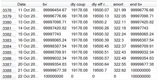
Here are the last few rows in the table.
|
Date
|
Book value
|
daily coupon
|
daily effective rate
|
amortization
|
Ending book value
|
|
10/13/2019
|
99996776.65841
|
19178.08219
|
19500.13378
|
322.0516
|
99997098.71001
|
|
10/14/2019
|
99997098.71001
|
19178.08219
|
19500.19659
|
322.1144
|
99997420.82440
|
|
10/15/2019
|
99997420.82440
|
19178.08219
|
19500.2594
|
322.1772
|
99997743.00161
|
|
10/16/2019
|
99997743.00161
|
19178.08219
|
19500.32223
|
322.24
|
99998065.24165
|
|
10/17/2019
|
99998065.24165
|
19178.08219
|
19500.38507
|
322.3029
|
99998387.54452
|
|
10/18/2019
|
99998387.54452
|
19178.08219
|
19500.44792
|
322.3657
|
99998709.91025
|
|
10/19/2019
|
99998709.91025
|
19178.08219
|
19500.51078
|
322.4286
|
99999032.33884
|
|
10/20/2019
|
99999032.33884
|
19178.08219
|
19500.57366
|
322.4915
|
99999354.83031
|
|
10/21/2019
|
99999354.83031
|
19178.08219
|
19500.63655
|
322.5544
|
99999677.38466
|
|
10/22/2019
|
99999677.38466
|
19178.08219
|
19500.69945
|
322.6173
|
100000000.00192
|
|
Total
|
|
64975342.47
|
65775342.47
|
800000
|
|
We can see that the book value on 10/22/2019 reflects the face value of the bond and we can see that the total amortization of 800,000 is the difference between the clean price of the bond when it was purchased and the face value of the bond at maturity, as we would expect it to be.
Let’s look at how we would do this in SQL Server.
Our first real challenge is coming up with the daily effective rate. Remember, this was supplied to the EXCEL table through the use of the Solver function and we do not have a Solver function in SQL Server. But, do we really need one to come up with the rate?
When I look at the amortization table, it immediately strikes me that we can think of the table as consisting of a series of cash flows. The initial cash flow is the clean price of the bond, which we have recorded as the book value on 2010-07-13. The daily coupon can be thought of as a cash flow that is received every day from 2010-07-14 until the maturity date of the bond, 2019-10-22. Finally, on the maturity date, in addtion to the daily coupon, we receive the face amount. What would happen if we put all these dates and cash flows into the XIRR function?
Let’s declare our varaibles.
DECLARE @fa as float = 100000000
DECLARE @pr as float = 99200000
DECLARE @rt as float = .07
DECLARE @sd as datetime = '2010-07-13'
DECLARE @ed as datetime = '2019-10-22'
The following SQL, which uses the XLeratorDB table-valued function SeriesDate, will create all the cash flows described above.
SELECT SeriesValue
,CASE SeriesValue
WHEN @sd THEN -@pr --the clean price on the start date
WHEN @ed THEN (1 + @rt/365) * @fa --the maturity value on the end date
ELSE @rt/365 * @fa --the daily coupon
END
FROM wct.SeriesDate(@sd,@ed,NULL,NULL,NULL)
We can put the cash flows into a derived table and the use the XIRR function to calculate an effective rate.
SELECT wct.XIRR(cfamt,cfdate,NULL) as [Eff Rate]
FROM (
SELECT SeriesValue
,CASE SeriesValue
WHEN @sd THEN -@pr --the clean price on the start date
WHEN @ed THEN (1 + @rt/365) * @fa --the maturity value on the end date
ELSE @rt/365 * @fa --the daily coupon
END
FROM wct.SeriesDate(@sd,@ed,NULL,NULL,NULL)
) n(cfdate, cfamt)
This produces the following result.
Eff Rate
----------------------
0.0737646558138463
However, this is an annual rate and we need a daily rate. The following SQL will convert the annualized XIRR value into the equivalent daily rate that can be used for the amortization calculation.
SELECT POWER(1+wct.XIRR(cfamt,cfdate,NULL),1.0000/365.0000) - 1 as [Eff Rate]
FROM (
SELECT SeriesValue
,CASE SeriesValue
WHEN @sd THEN -@pr --the clean price on the start date
WHEN @ed THEN (1 + @rt/365) * @fa --the maturity value on the end date
ELSE @rt/365 * @fa --the daily coupon
END
FROM wct.SeriesDate(@sd,@ed,NULL,NULL,NULL)
) n(cfdate, cfamt)
This produces the following result.
Eff Rate
----------------------
0.000195007623567722
As you can see, this is the same rate that was used in the amortization schedule produced by EXCEL.
However, it is possible to actually simplify the calculation, by using the IRR function, as it will return the daily rate with no manipulation of the result.
SELECT wct.IRR(cfamt,seq,NULL) as [Eff Rate]
FROM (
SELECT seq
,CASE SeriesValue
WHEN @sd THEN -@pr --the clean price on the start date
WHEN @ed THEN (1 + @rt/365) * @fa --the maturity value on the end date
ELSE @rt/365 * @fa --the daily coupon
END
FROM wct.SeriesDate(@sd,@ed,NULL,NULL,NULL)
) n(seq, cfamt)
This produces the following result.
Eff Rate
----------------------
0.000195007623595922
The XIRR and IRR functions are designed for irregular cash flows. In other words, different periods may have different cash flows. We really only have three cash flows: the clean price, the daily coupon, and the face amount.
These three amounts fit very nicely into the RATE function, where the clean price is the present value amount, the daily coupon is the periodic payment amount, and the face amount is the future value. Thus, we can calculate the daily effective rate with the following very simple statement.
SELECT wct.RATE(DATEDIFF(d,@sd,@ed),@rt/365*@fa,-@pr,@fa,0,NULL) as [Eff Rate]
Which produces the following result.
Eff Rate
----------------------
0.000195007623595989
Now that we know the daily rate, we can produce the amortization schedule directly, by adding two more variables to our declarations.
DECLARE @np as int = DATEDIFF(d,@sd,@ed)
DECLARE @dr as float = wct.RATE(@np,@rt/365*@fa,-@pr,@fa,0,@rt/365)
Using the SeriesDate function, we can now produce the amortization schedule in SQL Server. Again, we will round the results to make the output easier to read.
SELECT convert(varchar, SeriesValue, 106) as Date
,ROUND(bv, 2) as bv
,ROUND([dly coup], 2) as [dly coup]
,ROUND([dly eff rate], 2) as [dly eff rate]
,ROUND([end bv] - bv,2) as amort
,ROUND([end bv], 2) as [end bv]
FROM (
SELECT Seq
,seriesvalue
,-wct.PV(@dr,@np-seq+1,@rt/365 * @fa,@fa,0) as bv
,@rt/365 * @fa as [dly coup]
,@dr * -wct.PV(@dr,@np-seq+1,@rt/365 * @fa,@fa,0) as [dly eff rate]
,-wct.PV(@dr,@np-seq,@rt/365 * @fa,@fa,0) as [end bv]
FROM wct.SeriesDate(@sd + 1,@ed,NULL,NULL,NULL)
UNION ALL
SELECT 0,@sd, @pr, 0,0,@pr
) a
ORDER BY SeriesValue
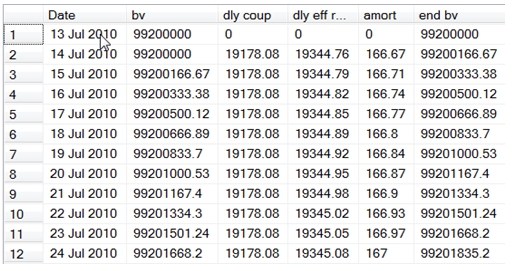
Here are the first few lines of the resultant table.
Here are the last few lines of the resultant table.
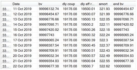
As you can see, the SQL produces the same results as our EXCEL table. Notice that the SQL is a single-pass solution, in that each row is self-contained. To achieve this, we have calculated the ending and beginning book values using the PV function and we calculated the amortization as the difference between the ending book value and the beginning book value. In order to keep the SQL simple, we have excluded the start date from the table-valued function and used a UNION ALL statement to put the start values into our derived table. If we wanted to create a schedule where the amortization and accruals were done on a first-not-last basis, we would make the following simple modifications to our SQL.
SELECT convert(varchar, SeriesValue, 106) as Date
,ROUND(bv, 2) as bv
,ROUND([dly coup], 2) as [dly coup]
,ROUND([dly eff rate], 2) as [dly eff rate]
,ROUND([end bv] - bv,2) as amort
,ROUND([end bv], 2) as [end bv]
FROM (
SELECT Seq
,seriesvalue
,-wct.PV(@dr,@np-seq+1,@rt/365 * @fa,@fa,0) as bv
,@rt/365 * @fa as [dly coup]
,@dr * -wct.PV(@dr,@np-seq+1,@rt/365 * @fa,@fa,0) as [dly eff rate]
,-wct.PV(@dr,@np-seq,@rt/365 * @fa,@fa,0) as [end bv]
/*FROM wct.SeriesDate(@sd + 1,@ed,NULL,NULL,NULL)*/
FROM wct.SeriesDate(@sd,@ed-1,NULL,NULL,NULL)
UNION ALL
/*SELECT 0,@sd, @pr, 0,0,@pr*/
SELECT @np,@ed, @fa, 0,0,@fa
) a
ORDER BY SeriesValue
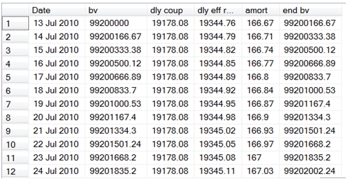
Here are the first few rows of the resultant table.
And, here are the last few rows.
If you remember, the interest basis for this calculation was actual/365. For loans that are actual/360 (i.e when the interest is accrued based on the actual number of days in the period divided by 360), we could simply change the number 365 to 360 in the SQL.
There are a couple on interesting things to note about this approach. First, we are completely unconcerend about the coupon frequency, and thus not concerned about when the coupon interest is actually received. That may not be an acceptable premise in your organization.
Second, we have assumed that the daily coupon amount is constant over the life of the bond. That may be OK with bonds that accrue on an actual/365 or actual/360 basis, but most bonds do not accrue interest that way. Generally, the coupon amounts for a bond are fixed and the daily interest may change from period to period. For example, a bond that that trades on a BOND or EBOND basis and has coupon payments twice a year will accrue 1/12th of the interest in each month, regardless of the number of days in the month. February, with 28 or 29 days will have the same accrued interest as March with 31 days.
I will now show you another approach to amortizing these bond that is very similar to the approach that we used for bonds that accrue on an actual/365 and actual 360 basis. This approach can only be used for bonds that accrue on a 30/360 basis.
Let’s set up our variables.
DECLARE @fa as float = 100000000 --face amount
DECLARE @pr as float = 99000000 --clean price
DECLARE @rt as float = .02 --coupon rate
DECLARE @sd as datetime = '2011-10-15' --start date
DECLARE @ed as datetime = '2013-10-15' --end date
DECLARE @np as int = -wctFinancial.wct.DAYS360(@ed,@sd,NULL) --number of periods
DECLARE @dc as float = @fa*@rt/360 --daily coupon
DECLARE @dr as float = wct.RATE(@np,@dc,-@pr,@fa,0,@rt/360) --effective rate
Notice that instead of calculating the number of periods as the difference in days between the start date and the end date, we are using the DAYS360 function to calculate the number of days. This is going to set the number of periods to 720 rather than 731, the actual number of days between the start date and the end date. This reflects the conventions associated with these kinds bonds. If you multiply the number of periods (@np) by the daily coupon (@dc) you will see that it correctly calculates 4,000,000, the amount of interest to paid on this bond over the life.
As we pointed out earlier, these bonds have the quirk of not accruing on the 31st of the month and accruing multiples of the daily coupon on the last day of February. We are going to use the DAYS360 function to determine when we need to do this.
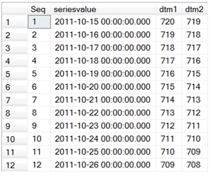
The first thing that I am going to do is generate all the dates that I need for this bond, and at the same time calculate the number of days to maturity for each date and the number of days to maturity for the next date for each date. I will put these in columns called dtm1 and dtm2.
SELECT Seq
,seriesvalue
,-wctFinancial.wct.DAYS360(@ed,SeriesValue,NULL) as dtm1
,-wctFinancial.wct.DAYS360(@ed,SeriesValue+1,NULL) as dtm2
FROM wct.SeriesDate(@sd,@ed-1,NULL,NULL,NULL)
Here are the first few rows of the resultant table.
We are going to use the difference between dtm1 and dtm2 in the calculation of the daily coupon and daily amortization amount. If we put this SQL in a derived table and add the following SQL around it, we can generate our amortization schedule quite easily. I am going to put the results into a temporary table, #a2, so that we can analyze the results without having to re-enter all the SQL. Again, I will round the results to make them easier to read.
SELECT a.SeriesValue
,wct.PV(@dr,dtm1,-@dc,-@fa,0) as bv
,@dc*(dtm1-dtm2) as [dly coup]
,wct.PV(@dr,dtm2,-@dc,-@fa,0) - wct.PV(@dr,dtm1,-@dc,-@fa,0) as [dly amort]
,wct.PV(@dr,dtm2,-@dc,-@fa,0) as [end bv]
INTO #a2
FROM (
SELECT Seq
,seriesvalue
,-wctFinancial.wct.DAYS360(@ed,SeriesValue,NULL) as dtm1
,-wctFinancial.wct.DAYS360(@ed,SeriesValue+1,NULL) as dtm2
FROM wct.SeriesDate(@sd,@ed-1,NULL,NULL,NULL)
) a
SELECT convert(varchar, a.SeriesValue, 106) as Date
,ROUND(a.bv, 2) as bv
,ROUND(a.[dly coup], 2) as [dly coup]
,ROUND(a.[dly amort], 2) as [dly amort]
,ROUND(a.[end bv], 2) as [end bv]
FROM #a2 a
ORDER BY a.SeriesValue
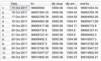
Here are the first few rows of the resultant table.
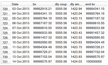
And here are the last few rows.
Everything looks pretty good. Let’s check to make sure the coupon interest and the amortization totals are correct.
SELECT ROUND(SUM(a.[dly coup]),4) as [Coupon Interest]
,ROUND(SUM(a.[dly amort]),4) as [Amortization]
FROM #a2 a
This produces the following result.
Coupon Interest Amortization
---------------------- ----------------------
4000000 1000000
Let’s see what happens on the last day of a month having 31 days.
SELECT convert(varchar, a.SeriesValue, 106) as Date
,ROUND(a.bv, 2) as bv
,ROUND(a.[dly coup], 2) as [dly coup]
,ROUND(a.[dly amort], 2) as [dly amort]
,ROUND(a.[end bv], 2) as [end bv]
FROM #a2 a
WHERE DAY(a.SeriesValue) = 31
This produces the following result.
This is also, what we would expect. Let’s look at what happens on the last day of February.
SELECT convert(varchar, a.SeriesValue, 106) as Date
,ROUND(a.bv, 2) as bv
,ROUND(a.[dly coup], 2) as [dly coup]
,ROUND(a.[dly amort], 2) as [dly amort]
,ROUND(a.[end bv], 2) as [end bv]
FROM #a2 a
WHERE Month(a.SeriesValue) = 2
AND a.SeriesValue = wct.CALCDATE(Year(SeriesValue),Month(seriesValue) + 1, 1) - 1
This produces the following result.
Again, this is what we would expect. We accrued 2 days interest and 2 days of amortization on the last day of February in 2012, and 3 days on the last day of February 2013.
We can also double-check to make sure that we are, in fact, holding the rate constant.
SELECT convert(varchar, a.SeriesValue, 106) as Date
,ROUND(a.bv, 2) as bv
,ROUND(a.[dly coup], 2) as [dly coup]
,ROUND(a.[dly amort], 2) as [dly amort]
,ROUND(a.[end bv], 2) as [end bv]
,cast((a.[dly amort] + a.[dly coup]) / bv as Decimal(18,12)) as [Eff Rate]
FROM #a2 a
Here are the first few rows in the resultant table.
And here are the last few rows.
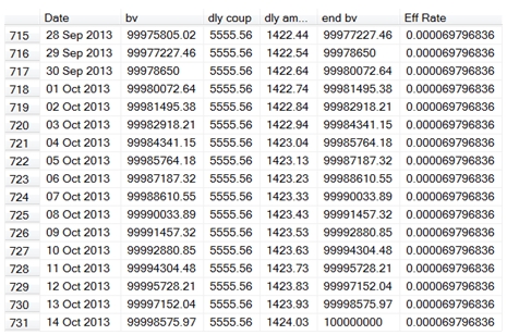
As you can see, the effective rate is the same at the end of amortization period as it is at the beginning of the amortization period. Of course, on the days when there is no coupon accrual there is no amortization, the effective rate is zero and on the last days of February the effective rate is approximately double or triple.
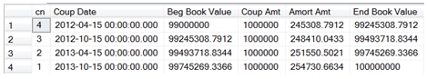
How does this line up with amortization based on the coupon dates?
SELECT cn
,Dateadd(d,1,MAX(SeriesValue)) as [Coup Date]
,ROUND(MIN(bv), 4) as [Beg Book Value]
,ROUND(SUM([dly coup]), 4) as [Coup Amt]
,ROUND(SUM([dly amort]), 4) as [Amort Amt]
,ROUND(MAX([end bv]), 4) as [End Book Value]
FROM (
SELECT a.*
,wct.COUPNUM(a.seriesValue,@ed,2,0) as cn
FROM #a2 a
) b
GROUP BY cn
ORDER BY 1 desc
This produces the following result.
And we can use our SQL from the beginning of the article to calculate the amortization holding the yield constant.
DECLARE @s as datetime = '2011-10-15' --settlement date
DECLARE @m as datetime = '2013-10-15' --maturity date
DECLARE @rt as float = .02 --coupon rate
DECLARE @fa as float = 100000000 --face amount
DECLARE @pr as float = 99000000 --proceeds
DECLARE @rn as float = 100 --redemption
DECLARE @f as float = 2 --frequency
DECLARE @b as nvarchar(1) = 0 --basis
DECLARE @y as float =(SELECT wct.YIELD(@s,@m,@rt,@pr/@fa*100,@rn,@f,@b)) --yield
DECLARE @nc as float =(SELECT wct.COUPNUM(@s,@m,@f,@b)) --number of coupons
SELECT c_num
,c_date
,coup * @fa/100 as coup
,amort * @fa/100 as amort
,bv * @fa/100 as bv
FROM (
SELECT Seq as c_num
,convert(varchar, wct.EDATE(@m,-Seriesvalue*12/@f), 106) as c_date
,100 * @rt/@f as coup
,wct.PRICE(wct.EDATE(@m,-Seriesvalue*12/@f),@m,@rt,@y,@rn,@f,@b) - wct.PRICE(wct.EDATE(@m,-(Seriesvalue+1)*12/@f),@m,@rt,@y,@rn,@f,@b) as amort
,wct.PRICE(wct.EDATE(@m,-Seriesvalue*12/@f),@m,@rt,@y,@rn,@f,@b) as bv
FROM wct.SeriesInt(@nc-1,0,NULL,NULL,NULL)
UNION ALL
SELECT 0, convert(varchar,@s,106),0,0,@pr/@fa * 100 --the value of the bond at the start
) c
ORDER BY 1
This produces the following result.
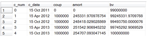
As you can see the results are very similar. Or, in accounting speak, you might say that the differences are immaterial.
This just leaves the case of actual/actual bonds, which should be treated the same way as actual/365 bonds.
No matter which technique is used, once we have generated the daily schedules, we can then summarize them into any period(s) that we want.
Regardless of which technique you are going to use for bond amortization in your own organization, having such a wide variety of functions on the database provides you with an enormous amount of flexibility as well making things easier. You can standardize calculations within your organization, and enforce that standardization by putting everything into the database. And since you are doing the calculations in the database, store the results there, too, so that everybody is using the same data, too. Eliminate all risk and effort associated with doing these types of calculations in a spreadsheet.