The case against Treasury Bonds
Sep
3
Written by:
Charles Flock
9/3/2010 8:13 AM

Are Treasury Bonds really a risk free investment?
In reading the financial press, I am always struck by the use of phrases like ‘flight to safety’ and ‘risk-free’. In particular, there is a lot of press about a bubble in the bond market and about investors taking money out of equities and buying the 10-year or 30-year Treasury bond. Today we are going to look at the mechanics of bond pricing and see how movements in the bond market affect your returns.
As I write this, the ‘on-the-run’ 10-year note has a maturity date of 8/15/2020 and a coupon rate of 2.625%, which means that every 6 months (on 2/15 and 8/15) the US Treasury will send you a check for $1.3125 for every $100 in face value of bonds that you own. Think of the bond as a stream of payments of $1.3125 with an additional $100 paid at the maturity date. As I write this, the bond is trading at a price of 100-02+ which, in decimal terms, is 100.078125. This piece of SQL tells us the important statistics about the bond:
SELECT 100 + cast(2.5 as float)/cast(32 as float) as PRICE
,wct.YIELD('09/03/2010'
,'08/15/2020'
,.02625
,100 + cast(1.5 as float)/cast(32 as float)
, 100
,2
,1) as YIELD
,wct.BONDINT('09/03/2010'
,'08/15/2020'
,.02625
,100
,2
,1) AS [ACCRUED INTREREST]
,100 + cast(1.5 as float)/cast(32 as float) +
wct.BONDINT('09/03/2010'
,'08/15/2020'
,.02625
,100
,2
,1) AS [CASH OUTLAY]
This returns the following result.
PRICE YIELD ACCRUED INTREREST CASH OUTLAY
---------------------- ---------------------- ---------------------- ----------------------
100.078125 0.0261952631692048 0.135529891304348 100.182404891304
(1 row(s) affected)
Since the price of the bond is greater than 100 (the par value of the bond being 100), then the yield of the bond is (generally) less than the coupon (or interest) rate of the bond. Additionally, since the bond was issued on 8/15/2010 and we are buying it for settlement 9/3/2010, a portion of the interest (called the Accrued Interest) is paid by the buyer of the bond to the seller of the bond, since the buyer will receive the coupon interest from the issuer at a later date. Buying the bond, then, requires a cash outlay of $100.1824, which is called the ‘dirty’ price.
What am I getting for this $100.1824? A series of semi-annual coupons of $1.3125 and a final payment of $100 on 8/15/2020 and the complete confidence that the US government will actually satisfy its obligations. But, does that mean that there is no risk?
Let’s look at a couple of things that might affect our thinking. First, what if something unexpected happens in a year and I need to convert the bond to cash? Since the US Treasury market is highly liquid, it is generally no problem to sell a bond. However, the price and yield of the bond are directly linked in the following way: as prices go up, yields go down; as prices go down, yields go up. Which is why saying things like ‘interest rates are going down because bond prices are up’ is a statement that doesn’t really tell you anything.
Is there any way to know what interest rates will be doing a year from now? Not really. Nevertheless, there are some interesting things to think about. With the yield at 2.62%, bonds are near their historic low. In the last 50 years, the low yield for 10-Year Treasury Constant Maturity is 2.08%, which happened on 12/18/2008. The high is 15.84%, which happened on 9/30/1981. Interestingly enough, both instances occurred during recessions.
With this little piece of SQL, we can look at possible outcomes of our investment in one-year’s time at yields from 2% to 5%:
SELECT n.*
,[DIRTY PRICE] - 100 + cast(1.5 as float)/cast(32 as float) +
wct.BONDINT('09/03/2010'
,'08/15/2020'
,.02625
,100
,2
,1) + 2.625 as [PROFIT]
FROM (
SELECT seriesvalue as YIELD
,wct.PRICE(dateadd(YY, 1, '09/02/2010')
,'08/15/2020'
,.02625
,seriesvalue
,100
,2
,1) as PRICE
,wct.PRICE(dateadd(YY, 1, '09/02/2010')
,'08/15/2020'
,.02625
,seriesvalue
,100
,2
,1) +
wct.BONDINT(dateadd(YY, 1, '09/02/2010')
,'08/15/2020'
,.02625
,100
,2
,1) AS [DIRTY PRICE]
from wct.SeriesFloat(.020, .05, .001, NULL, NULL)
) n
This produces the following result:
YIELD PRICE DIRTY PRICE PROFIT
---------------------- ---------------------- ---------------------- ----------------------
0.02 105.098440363219 105.226837102349 8.03424199365371
0.021 104.263153640996 104.391550380126 7.19895527143034
0.022 103.435364674033 103.563761413164 6.37116630446822
0.023 102.61500134825 102.74339808738 5.55080297868446
0.024 101.801992283003 101.930389022133 4.73779391343784
0.025 100.99626682325 101.124663562381 3.93206845368525
0.026 100.197755031795 100.326151770925 3.1335566622295
0.027 99.406387681617 99.5347844207475 2.34218931205183
0.028 98.6220962482975 98.750492987428 1.55789787873232
0.029 97.8448129025166 97.973209641647 0.780614532951379
0.03 97.074470502644 97.2028672417744 0.0102721330787467
0.031 96.3110025874083 96.4393993265387 -0.753195782156961
0.032 95.5543433686504 95.6827401077808 -1.50985500091482
0.033 94.8044277241547 94.9328244632851 -2.25977064541057
0.034 94.0611911905628 94.1895879296932 -3.00300717900245
0.035 93.3245699563653 93.4529666954958 -3.73962841319988
0.036 92.594500854973 92.7228975941034 -4.46969751459222
0.037 91.8709213578617 91.9993180969921 -5.19327701170353
0.038 91.1537695677973 91.2821663069278 -5.91042880176787
0.039 90.4429842121341 90.5713809512646 -6.62121415743107
0.04 89.738504636189 89.8669013753194 -7.32569373337622
0.041 89.0402707966867 89.1686675358171 -8.02392757287852
0.042 88.3482232552809 88.4766199944114 -8.7159751142843
0.043 87.6623031721453 87.7906999112757 -9.40189519741991
0.044 86.9824522996375 87.110849038768 -10.0817460699277
0.045 86.3086129760305 86.4370097151609 -10.7555853935347
0.046 85.6407281193162 85.7691248584466 -11.423470250249
0.047 84.9787412210763 85.1071379602067 -12.0854571484889
0.048 84.3225963404227 84.4509930795531 -12.7416020291425
0.049 83.6722380980014 83.8006348371318 -13.3919602715638
0.05 83.0276116700668 83.1560084091973 -14.0365866994984
(31 row(s) affected)
We can ship these results off to EXCEL and create a nice little chart:

So if rates stay under 3%, it’s possible to sell the bond in one year and still make a profit, including the coupon interest. I can’t really speculate about where interest rates will be in one-year’s time, but I thought it would be kind of interesting to know how interest rates have behaved historically, so I downloaded the 10-year constant maturity rate data from the St. Louis Fed (http://research.stlouisfed.org/fred2/series/DGS10?cid=115) into SQL Server and did a little analysis of the data. I create a table, DGS10, which contains the data from the St. Louis Fed and discarded all the rows that were NULL (of which there were a surprising number).
SELECT YIELD, COUNT(*)
FROM DGS10
WHERE YIELD IS NOT NULL
GROUP BY YIELD
ORDER by 1 ASC
I took the result of this SELECT and graphed them. All this is giving me is a dispersal of the data points in the dataset. This is what the graph looks like:
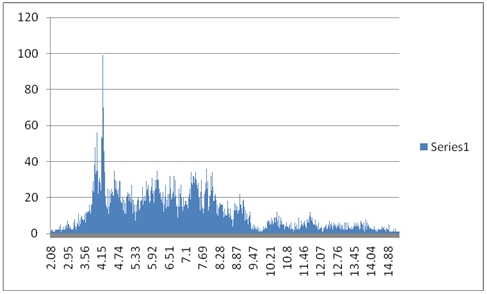
As you can see, it is a relative rare occurrence for the 10-year rate to be under 3.56%, and the fattest part of the graph is in the region between about 4.0% and 8.0%. It’s also quite obvious that the data are not normally distributed, so it’s probably not meaningful to look at things like standard deviation and average to come to some understanding of the data. However, we can use the PERCENTILE function to get some interesting insight
SELECT wct.Percentile_q('SELECT YIELD FROM DGS10',.025)
,wct.Percentile_q('SELECT YIELD FROM DGS10',.975)
This produces the following result:
---------------------- ----------------------
3.47 13.58
(1 row(s) affected)
This tells us that 95.0% of the time the YIELD value contained in the dataset is between 3.47% and 13.58%, which is a pretty big range. But, interestingly enough, the yield on the bond today is aproximately 85 basis points below the bottom of that range. Not a very encouraging statistic.
Next let’s look at what the biggest year over year change in rates has been. I ran the following statement:
SELECT a.date as start_date
,a.YIELD as start_yield
,b.date as end_date
,b.YIELD as end_yield
,ROUND(B.YIELD - A.YIELD, 2) as delta_YIELD
FROM DGS10 a, DGS10 b
WHERE b.date = wct.EDATE(a.date, 12)
AND A.YIELD IS NOT NULL
AND B.YIELD IS NOT NULL
And put the results into the following graph:
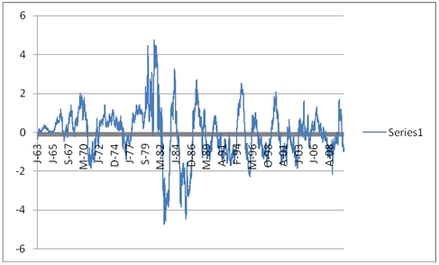
This graph shows the change in the 10-year yield after one-year. Notice that big up years tend to be followed by big down years. Notice also that the 21st century is a lot less volatile than other parts of the graph, but at the moment we are in a downward position on the graph implying that in the future, yields will go up (which is bad for the price of the bond).
Now that I have my data in SQL Server and I can use the XLeratorDB functions to perform really an unlimited number of analyses on bond performance, which should enhance my ability to make investment decisions. The analysis here leads me to believe that over the next year, I don’t want to own the 10-year bond.