Calculating Life Expectancy in SQL Server
Nov
27
Written by:
Charles Flock
11/27/2009 4:36 PM

How a simple function like PRODUCT can profoundly change the capabilities of T-SQL
Sometimes I just can’t help myself. With all the discussion about the ‘health bills’ (aren’t they really insurance bills?) in the news media, I got to wondering exactly what it is the US government is buying for the trillions of dollars that it is proposing to spend. Wouldn’t you know it; the Sunday NY Times magazine just ran a cover story, Making Health Care Better. This interesting article about Dr. Brent James and evidence-based medicine makes the point that life expectancy in 1910 was less than 50 years and that today it is over 78 years. It seems obvious, then, that one way of measuring the effectiveness ‘health care reform’ is to evaluate the impact on life expectancy.
Generally, life expectancy information is presented as a table, which allows you to look up how many more years a person of a certain age can expect to live. It looks like the type of calculation that lends itself to a spreadsheet. Today we will explore whether or not it makes sense to consider having this calculation done on the database rather than exporting data to EXCEL and doing the calculation there.
Life expectancy in humans is the average number of years of life remaining for people of a given age, assuming that everyone will experience, for the remainder of their lives, the risk of death based on a current life table. Here is an example of a current life table from the Office of National Statistics (ONS) in the UK.
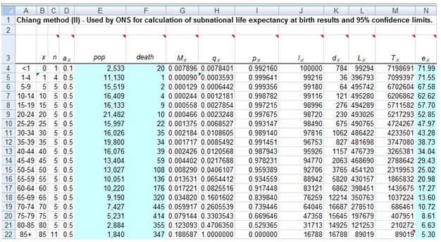
Cell N4 contains the life expectancy at birth, 71.99 years. The data provided to the calculation are in the range E4:F22 highlighted in blue. The range G4: N22 contains formulae. The range A4:D22 contains constants, with the exception of cell C22, which contains a formula for calculation the value n for the final age interval.
Before going into the mechanics of this calculation and its implementation in T-SQL, let’s discuss the rationale for doing so. After all, we have a perfectly good spreadsheet that calculates life expectancy quite nicely.
Life expectancy is calculated for a variety of different populations. In the US, for example, we calculate life expectancy for the country, for men and women, for a variety of ethnic classifications, for men and women in those ethnic classifications, and potentially in a number of other ways: by geography; by educational attainment; etc. Moreover, we keep track of something like 133 different classifications of death, which are generally summarized into 15 different categories. It’s easy to imagine several hundred or even a thousand different spreadsheets with life expectancy calculations in them.
By moving the calculation into T-SQL, all the calculations are in one place, and it simply becomes a matter of selecting the population data included in the calculation, allowing the analysis of unlimited dimensions. You also gain the advantage of the calculation being fast, secure, easily audited, and being sure that the data has not been manipulated in any way. For the purposes of this article, I am going to keep the calculation as simple as possible, but it is not for the faint of heart, even though it doesn’t require much math. I have chosen the ONS table as an example, because it breaks out all the parts of the calculation quite nicely, but you can find similar tables at National Center for Health Statistics web site.
Let’s start by creating a table. In this example, I have used a temporary table, but there is no reason that it should not be a permanent table.
Create table #l (
seq int,
descr varchar(5),
x int, --width of the age interval
n float, --population in age interval
a_x float, --Fraction of the age interval lived by those in the cohort population who die in the interval
pop float, --population in the age interval
death float, --number of deaths in the age interval
M_x as death/pop, --age-specific death rate
rate
Q_x as CASE
WHEN descr like '%+' THEN 1
ELSE n*(death/pop)/(1+n*(1-a_x)*(death/pop))
END, --Conditional probablity that an indivdual who has survived to start of the age interval will die in the age interval
P_x as CASE
WHEN descr like '%+' THEN 0
ELSE 1 - (n*death/pop)/(1+n*(1-a_x)*death/pop)
END --Conditional probablity that an indivdual entering the age interval will survive the age interval
)
As you can see, the columns M_x, Q_x, and P_x are computed columns, since there value is dependent on the other columns in the row.
We can than insert the data from the EXCEL spreadsheet into the table that we just created:
INSERT INTO #l VALUES (1, '<1',0,1,0.1,2533,20)
INSERT INTO #l VALUES (2, '1-4',1,4,0.5,11130,1)
INSERT INTO #l VALUES (3, '5-9',5,5,0.5,15519,2)
INSERT INTO #l VALUES (4, '10-14',10,5,0.5,16409,4)
INSERT INTO #l VALUES (5, '15-19',15,5,0.5,16133,9)
INSERT INTO #l VALUES (6, '20-24',20,5,0.5,21482,10)
INSERT INTO #l VALUES (7, '25-29',25,5,0.5,15997,22)
INSERT INTO #l VALUES (8, '30-34',30,5,0.5,16026,35)
INSERT INTO #l VALUES (9, '35-39',35,5,0.5,19800,34)
INSERT INTO #l VALUES (10, '40-44',40,5,0.5,16076,39)
INSERT INTO #l VALUES (11, '45-49',45,5,0.5,13404,59)
INSERT INTO #l VALUES (12, '50-54',50,5,0.5,13027,108)
INSERT INTO #l VALUES (13, '55-59',55,5,0.5,10051,136)
INSERT INTO #l VALUES (14, '60-64',60,5,0.5,10220,176)
INSERT INTO #l VALUES (15, '65-69',65,5,0.5,9190,320)
INSERT INTO #l VALUES (16, '70-74',70,5,0.5,7427,445)
INSERT INTO #l VALUES (17, '75-79',75,5,0.5,5231,414)
INSERT INTO #l VALUES (18, '80-85',80,5,0.5,2884,355)
INSERT INTO #l VALUES (19, '85+',85,10.6051873198847,0.5,1840,347)
The following calculations require the values from more than one row, so we will use a common table expression. This SELECT will recreate all the data contained in the EXCEL spreadhseet.
;with mycte as (
select l1.*
,CASE
WHEN l1.x = 0 THEN 100000
ELSE wct.PRODUCT(l2.P_X) * 100000
END as l_x --Life table cohort population.
--The hypothetical population of newborn babies on which the life table is based.
--This is usually defined as 100,000 as in this example.
,CASE
WHEN l1.x = 0 THEN 100000
ELSE wct.PRODUCT(l2.P_X) * 100000
END * l1.Q_x as d_x --Number of life table deaths in the age interval
,(CASE
WHEN l1.x = 0 THEN 100000
ELSE wct.PRODUCT(l2.P_X) * 100000
END - ((CASE
WHEN l1.x = 0 THEN 100000
ELSE wct.PRODUCT(l2.P_X) * 100000
END * l1.Q_x) * (1-l1.a_x))) * l1.n as Lx -- Number of years lived lived during the age interval
from #l l1, #l l2
where l2.seq < l1.seq or l1.seq = 1
group by l1.seq
,l1.descr
,l1.x
,l1.n
,l1.a_x
,l1.pop
,l1.death
,l1.M_x
,l1.Q_x
,l1.P_x) Select m1.seq
,m1.descr
,m1.x
,m1.n
,m1.a_x
,m1.pop
,m1.death
,m1.M_x
,m1.Q_x
,m1.P_x
,m1.l_x
,m1.d_x
,m1.Lx
,sum(m2.lX) as T_x --Cumulative number of years lived by the cohort population in the age interval and all subsequent age intervals.
,sum(m2.lX)/m1.l_x as ex --Life expectancy at the beginning of the age interval.
from MYCTE m1, mycte m2
where m2.seq >= m1.seq
group by m1.seq
,m1.l_x
,m1.descr
,m1.x
,m1.n
,m1.a_x
,m1.pop
,m1.death
,m1.M_x
,m1.Q_x
,m1.P_x
,m1.l_x
,m1.d_x
,m1.Lx
order by seq
When we run this SQL, we get the following result:
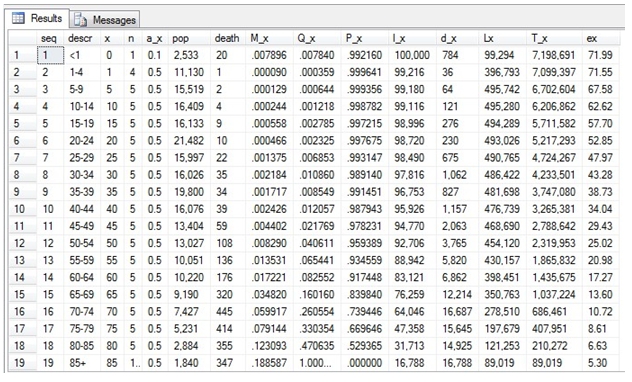
As you can see, we have produced exactly the same results as the EXCEL calculation.
The life expectancy calculation is interesting because the value of ex requires the summation of values ascending by age cohort and then the summation of values descending by age cohort. If you look at the l_x column, you can see that the value for every row after the initial row is dependent on the value in the preceding row. However, by using the PRODUCT function, we can calculate the value of l_x for any cohort directly from the underlying data. If we wanted to know the value l_x for the 60–64 cohort, that can be calculated directly using:
select wct.PRODUCT(1-Q_X) * 100000
from #l
where seq < 14
Which returns the following result:
----------------------
83121.1615948861
(1 row(s) affected)
The value of l_x is the number of people in the cohort at the start of the interval. The value of d_x is the number of life table deaths over the course of the interval. Thus, the value of d_x is simply the difference between the value of l_x for this cohort and the value of l_x for the next cohort. Once again, we can calculate this number directly.
select (wct.PRODUCT(1-l1.Q_X) - (wct.PRODUCT(1-l1.Q_X) * (1-l2.Q_X))) * 100000
from #l l1, #l l2
where l1.seq < 14
and l2.seq = 14
group by l2.Q_x
Which returns the following result:
----------------------
6861.78444685739
(1 row(s) affected)
Knowing l_x and d_x, we have enough information to calculate the value of Lx, the number of lives lived during the age interval. This calculation is l_x minus d_x multiplied by a_x multiplied by n.
select ((wct.PRODUCT(1-l1.Q_X) - (wct.PRODUCT(1-l1.Q_X) - (wct.PRODUCT(1-l1.Q_X) * (1-l2.Q_X)))* l2.a_x) * 100000) * l2.n
from #l l1, #l l2
where l1.seq < 14
and l2.seq = 14
group by l2.Q_x
,l2.a_x
,l2.n
Which returns the following result:
----------------------
398451.346857287
(1 row(s) affected)
This is where it gets interesting. To calcuate the life expectancy for this cohort (60–64), we need to know what Lx is for all the remaining cohorts, i. e. all the cohorts greater than or eqaul to this one. Calculating the Lx value for each cohort is straightforward.
select l2.seq
,((wct.PRODUCT(1-l1.Q_X) - (wct.PRODUCT(1-l1.Q_X) - (wct.PRODUCT(1-l1.Q_X) * (1-l2.Q_X)))* l2.a_x) * 100000) * l2.n as Lx
from #l l1, #l l2
where l1.seq < l2.seq
and l2.seq >= 14
group by l2.Q_x
,l2.a_x
,l2.n
,l2.seq
Which returns the following result:
seq Lx
----------- ----------------------
14 398451.346857287
15 350762.600595788
16 278509.947755464
17 197679.022548871
18 121252.998851995
19 89019.4467463805
(6 row(s) affected)
All we need to do is calculate the sum of Lx and divide it by l_x (isn’t that confusing) and we can get the life expectancy for the cohort. While that seems clear enough, it becomes a little tricky because the PRODUCT and SUM functions are aggregate functions. We cannot calculate an aggregate that includes an aggregate. One very simple way to overcome this limitation is to use a common table expression (CTE). Our CTE looks like this:
with mycte as (select l2.seq
,wct.PRODUCT(1-l1.Q_X) * 100000 as l_x
,((wct.PRODUCT(1-l1.Q_X) - (wct.PRODUCT(1-l1.Q_X) - (wct.PRODUCT(1-l1.Q_X) * (1-l2.Q_X)))* l2.a_x) * 100000) * l2.n as Lx
from #l l1, #l l2
where l1.seq < l2.seq
group by l2.Q_x
,l2.a_x
,l2.n
,l2.seq)
select sum(m2.Lx)/m1.l_x as ex
from mycte m1, mycte m2
where m2.seq >= m1.seq
and m1.seq = 14
group by m1.l_x
Which returns the following result:
ex
----------------------
17.2720801274764
(1 row(s) affected)
We have assigned each cohort a sequential number (seq) and we have a single SELECT statement that will calculate the value for any of the cohorts 2 through 19. The first row (seq = 1) represents a special case which we need to include in the CTE. There are many ways to do this and I have chosen UNION ALL since it makes it clear how the values for the first sequence are calculated.
with mycte as (select l2.seq
,wct.PRODUCT(1-l1.Q_X) * 100000 as l_x
,((wct.PRODUCT(1-l1.Q_X) - (wct.PRODUCT(1-l1.Q_X) - (wct.PRODUCT(1-l1.Q_X) * (1-l2.Q_X)))* l2.a_x) * 100000) * l2.n as Lx
from #l l1, #l l2
where l1.seq < l2.seq
group by l2.Q_x
,l2.a_x
,l2.n
,l2.seq
UNION ALL
select 1
,100000 as l_x
,100000*(1-(l1.Q_X * (1-l1.a_X)))
from #l l1, #l l2
where l1.seq = 1 and l2.seq = 2)
select sum(m2.Lx)/m1.l_x as ex
from mycte m1, mycte m2
where m2.seq >= m1.seq
and m1.seq = 1
group by m1.l_x
This returns the following result:
ex
----------------------
71.9869136892019
(1 row(s) affected)
Now, we can calculate the value for any age cohort.
Doing this type of calculation in SQL Server gives rise to several major advantages over exporting the data and doing the calculation in EXCEL.
1. We have eliminated any dependency on the physical layout of the data. The EXCEL calculation will only work if there are exactly 19 rows of data and if the data are sorted correctly. Additionally, there are different calculations for the first and last row if the calculation. If the number of rows changes or the data are not in order, then the spreadsheet needs to be changed, which is time-consuming and error prone.
2. We can analyze many different populations in a single unit of work without having to set up a different worksheet for each one. By using the spreadsheet as an analytical tool, we need to have a different worksheet or workbook for each demographic that is being analyzed. In the US, statistics are produced for 5 different ethnological classifications, and within each one, for both sexes, male, and female. That’s 15 different worksheets. It’s easy to imagine driving that analysis in other dimensions like standard metropolitan statistical area, or by educational attainment. You could end up with thousands of worksheets or workbooks.
3. Simplicity. Using T-SQL we were able to calculate the life expectancy for every cohort with 20 lines of SQL, containing 5 formulae. The equivalent EXCEL worksheet contains 152 formulae.
4. Only one instance of the data; no synchronization problems. Since we are using the database directly, we don’t have to worry about exporting the data to EXCEL; we are always using the most current version of the data.
5. Consistency is assured. Since we use the same SELECT statement for each population, we can feel comfortable that all results were calculated the same way. Since we are using T-SQL we can enforce that consistency by creating VIEWs which embody the SELECT statement or by putting the SELECT into a stored procedure or user-defined functions. In EXCEL, the formulae are physically copied into each cell in each worksheet, requiring tedious double-checking to avoid replicative failure.