Exploring the Time-weighted Rate of Return calculation in SQL Server
Oct
5
Written by:
Charles Flock
10/5/2017 9:56 PM

In this article we take a deeper look into the XLeratorDB TWRR function which is a very easy-to-use aggregate function for calculating time-weighted rate-of-return in SQL Server. But, easy-to-use doesn’t necessarily mean easy to understand. In this article we take a deeper look into the mechanics of the calculation.
TWRR implements the following formula for the calculation of time-weighted rate-of-return.
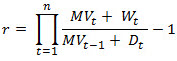
For each time interval (t) in period containing n time intervals calculate the return (rt) at time (t) as the ending market value plus withdrawals from the account divided by the beginning market value plus deposits into the account. Then calculate the product of all the rt values and subtract 1.
The aggregate function TWRR takes 3 columns as input: the date of the cash flow, the amount of the cash flow, and a bit value identifying the cash flows as a market value or not. When the bit value is 0, cash flow amounts greater than zero are treated as deposits (D) and cash flow amounts less than zero are treated as withdrawals (W). When the bit value is 1, cash flow amounts less than zero are treated as ending market values and cash flow amounts greater than zero are treated as beginning market values.
Let’s look at the calculation of time-weighted rate-of-return when the market values are the beginning market values. We will assume that the customer opens an account on 01-Jun-2017 with a deposit of 150,000. We will have a beginning market value for each day (and obviously we will be missing one for the first day, because that’s that day that the account was opened) and there will be several other transactions across the account from 01-Jun-2017 to 01-Sep-2017.
We identify the market values by setting mv = 1. Since they are going to calculated as beginning market values they will be positive. Deposits into the account will also be positive, while withdrawals will be negative. Both deposits and withdrawals will have mv = 0.
We will put the data into temp table, #cf.
SELECT
*
INTO
#cf
FROM (VALUES
('2017-06-01',NULL,1),('2017-06-01',150000,0)
,('2017-06-02',149803.89,1)
,('2017-06-05',149617.04,1)
,('2017-06-06',149489.24,1)
,('2017-06-07',149284.93,1)
,('2017-06-08',149405.33,1)
,('2017-06-09',149447.78,1)
,('2017-06-12',149620.57,1),('2017-06-12',-75000,0)
,('2017-06-13',74679.62,1)
,('2017-06-14',74756.75,1)
,('2017-06-15',74747.43,1)
,('2017-06-16',74795.3,1)
,('2017-06-19',74914.4,1)
,('2017-06-20',74929.78,1)
,('2017-06-21',74969.78,1)
,('2017-06-22',74987.43,1),('2017-06-22',25000,0)
,('2017-06-23',99937.46,1)
,('2017-06-26',100045.24,1)
,('2017-06-27',100092.94,1)
,('2017-06-28',100119.24,1)
,('2017-06-29',100126.82,1)
,('2017-06-30',100345.15,1)
,('2017-07-03',100337.07,1),('2017-07-03',-15000,0)
,('2017-07-04',85353.88,1)
,('2017-07-05',85307.15,1)
,('2017-07-06',85383.39,1)
,('2017-07-07',85449.07,1)
,('2017-07-10',85442.12,1)
,('2017-07-11',85366.81,1)
,('2017-07-12',85427.62,1)
,('2017-07-13',85244.71,1),('2017-07-13',-82500,0)
,('2017-07-14',2740.96,1)
,('2017-07-17',2739.91,1)
,('2017-07-18',2742.3,1)
,('2017-07-19',2746.64,1)
,('2017-07-20',2749.79,1),('2017-07-20',75000,0)
,('2017-07-21',77752.69,1)
,('2017-07-24',77781.27,1)
,('2017-07-25',77811.4,1)
,('2017-07-26',77960.14,1)
,('2017-07-27',77838.42,1)
,('2017-07-28',77893.44,1),('2017-07-28',25000,0),('2017-07-28',-10000,0)
,('2017-07-31',92883.74,1)
,('2017-08-01',93038.94,1)
,('2017-08-02',93013.21,1)
,('2017-08-03',92921.64,1)
,('2017-08-04',92884.4,1)
,('2017-08-07',92791.55,1)
,('2017-08-08',92951.07,1)
,('2017-08-09',92928.92,1)
,('2017-08-10',92939.06,1)
,('2017-08-11',93034.94,1)
,('2017-08-14',93170.69,1)
,('2017-08-15',93172.78,1)
,('2017-08-16',93008.48,1)
,('2017-08-17',92932.19,1)
,('2017-08-18',92848.9,1)
,('2017-08-21',92786.68,1)
,('2017-08-22',92811.25,1)
,('2017-08-23',92909.75,1)
,('2017-08-24',93027.99,1)
,('2017-08-25',93145.59,1)
,('2017-08-28',93298.38,1)
,('2017-08-29',93431.38,1)
,('2017-08-30',93509.65,1)
,('2017-08-31',93496.32,1)
,('2017-09-01',93595.27,1)
)n(dt,amt,mv)
Absolutely the simplest way to calculate the time-weighted rate-of-return for this data is to use the XLeratorDB TWRR function.
SELECT
wct.TWRR(amt, dt, mv) as [TWRR]
FROM
#cf
This produces the following result.
Let’s look at how that number is calculated. To do this, I am going to take the data in the #cf table and turn it into a spreadsheet format. The following SQL is one way to that.
SELECT
dt,
amt as BMV,
0 as D,
0 as W
FROM
#cf
WHERE
mv = 1
UNION ALL
SELECT
dt,
0 as BMV,
amt as D,
0 as W
FROM
#cf
WHERE
mv = 0 and amt > 0
UNION ALL
SELECT
dt,
0 as BMV,
0 as D,
-amt as W
FROM
#cf
WHERE
mv = 0 and amt < 0
While this will put the #cf data into the 3 columns that I want for this example, it can return multiple rows for each date and I need to get to a single row for each date. This can easily be done using the SUM function.
SELECT
dt,
SUM(BMV) as BMV,
SUM(D) as D,
SUM(W) as W
FROM (
SELECT
dt,
amt as BMV,
0 as D,
0 as W
FROM
#cf
WHERE
mv = 1
UNION ALL
SELECT
dt,
0 as BMV,
amt as D,
0 as W
FROM
#cf
WHERE
mv = 0 and amt > 0
UNION ALL
SELECT
dt,
0 as BMV,
0 as D,
-amt as W
FROM
#cf
WHERE
mv = 0 and amt < 0
)n
GROUP BY
dt
This puts the #cf data into a format where I can now use the SQL Server LEAD function to calculate the daily return for the TWRR calculation. I am going to put the results of this SQL into a temp table, #t, for the next step in the calculation.
This is what should be in #t.
Now, it’s simply a matter of taking the product of all the [1+r] values using the XLeratorDB PRODUCT function.
SELECT
wct.PRODUCT([1+r]) -1 as [Manual Calculation]
FROM
#t
And we can see that this produces exactly the same result of the XLeratorDB TWRR function.
In this example, the D and W values from the previous example are exactly the same, but the market values are passed into the function as ending market values. Notice that the ending market value for 01-Jun-2017 is equal and opposite in value to the P amount for that date. As before we will put the data in the temp table #cf.
SELECT
*
INTO
#cf
FROM (VALUES
('2017-06-01',150000,0),('2017-06-01',-150000,1)
,('2017-06-02',-149803.89,1)
,('2017-06-05',-149617.04,1)
,('2017-06-06',-149489.24,1)
,('2017-06-07',-149284.93,1)
,('2017-06-08',-149405.33,1)
,('2017-06-09',-149447.78,1)
,('2017-06-12',-75000,0),('2017-06-12',-74620.57,1)
,('2017-06-13',-74679.62,1)
,('2017-06-14',-74756.75,1)
,('2017-06-15',-74747.43,1)
,('2017-06-16',-74795.3,1)
,('2017-06-19',-74914.4,1)
,('2017-06-20',-74929.78,1)
,('2017-06-21',-74969.78,1)
,('2017-06-22',25000,0),('2017-06-22',-99987.43,1)
,('2017-06-23',-99937.46,1)
,('2017-06-26',-100045.24,1)
,('2017-06-27',-100092.94,1)
,('2017-06-28',-100119.24,1)
,('2017-06-29',-100126.82,1)
,('2017-06-30',-100345.15,1)
,('2017-07-03',-15000,0),('2017-07-03',-85337.07,1)
,('2017-07-04',-85353.88,1)
,('2017-07-05',-85307.15,1)
,('2017-07-06',-85383.39,1)
,('2017-07-07',-85449.07,1)
,('2017-07-10',-85442.12,1)
,('2017-07-11',-85366.81,1)
,('2017-07-12',-85427.62,1)
,('2017-07-13',-82500,0),('2017-07-13',-2744.71,1)
,('2017-07-14',-2740.96,1)
,('2017-07-17',-2739.91,1)
,('2017-07-18',-2742.3,1)
,('2017-07-19',-2746.64,1)
,('2017-07-20',75000,0),('2017-07-20',-77749.79,1)
,('2017-07-21',-77752.69,1)
,('2017-07-24',-77781.27,1)
,('2017-07-25',-77811.4,1)
,('2017-07-26',-77960.14,1)
,('2017-07-27',-77838.42,1)
,('2017-07-28',25000,0) ,('2017-07-28',-10000,0) ,('2017-07-28',-92893.44,1)
,('2017-07-31',-92883.74,1)
,('2017-08-01',-93038.94,1)
,('2017-08-02',-93013.21,1)
,('2017-08-03',-92921.64,1)
,('2017-08-04',-92884.4,1)
,('2017-08-07',-92791.55,1)
,('2017-08-08',-92951.07,1)
,('2017-08-09',-92928.92,1)
,('2017-08-10',-92939.06,1)
,('2017-08-11',-93034.94,1)
,('2017-08-14',-93170.69,1)
,('2017-08-15',-93172.78,1)
,('2017-08-16',-93008.48,1)
,('2017-08-17',-92932.19,1)
,('2017-08-18',-92848.9,1)
,('2017-08-21',-92786.68,1)
,('2017-08-22',-92811.25,1)
,('2017-08-23',-92909.75,1)
,('2017-08-24',-93027.99,1)
,('2017-08-25',-93145.59,1)
,('2017-08-28',-93298.38,1)
,('2017-08-29',-93431.38,1)
,('2017-08-30',-93509.65,1)
,('2017-08-31',-93496.32,1)
,('2017-09-01',-93595.27,1)
)n(dt,amt,mv)
Again, the simplest way to calculate the time-weighted rate-of-return is to use the XLeratorDB TWRR function.
SELECT
wct.TWRR(amt,dt,mv) as TWRR
FROM
#cf
This produces the following result.
Since we are using ending market values rather than beginning market values, we will use the LAG function rather than the LEAD function to calculate the daily returns.
SELECT
*
,(EMV+W)/(D + LAG(EMV,1,0) OVER (ORDER BY dt ASC)) as [1+r]
INTO
#t
FROM (
SELECT
dt,
SUM(cast(D as float)) as D,
SUM(cast(W as float)) as W,
SUM(cast(EMV as float)) as EMV
FROM (
SELECT
dt,
-amt as EMV,
0 as D,
0 as W
FROM
#cf
WHERE
mv = 1
UNION ALL
SELECT
dt,
0 as EMV,
amt as D,
0 as W
FROM
#cf
WHERE
mv = 0 and amt > 0
UNION ALL
SELECT
dt,
0 as EMV,
0 as D,
-amt as W
FROM
#cf
WHERE
mv = 0 and amt < 0
)n
GROUP BY
dt
)p
This is what should be in #t
Once again, it’s simply a matter of taking the product of all the [1+r] values using the XLeratorDB PRODUCT function.
SELECT
wct.PRODUCT([1+r]) -1 as [Manual Calculation]
FROM
#t
And we can see that this produces exactly the same result of the XLeratorDB TWRR function.
Passing the in the market values as beginning market values or ending market values can have a pretty significant impact on the TWRR calculation. Using beginning market values, the TWRR was 1.705%; using ending market values it was 1.477%. This is, of course, an artifact of my data, since basically I flipped one set of market values into the other. What’s important is that the data are passed into the function in a manner that is consistent with how your organization calculates the time-weighted rate-of-return. Hopefully, this explanation has helped.
Looking for other ways to calculate time-weighted rate-of-return? Check out the GTWRR and TWROR functions. Looking for other financial calculations? Go the financial functions index where you will find more than 250 financial written specifically for SQL Server.
Want to try this out for yourself? Download the 15-day trial here. Something that you would like to see added to the product? Send us a note at support@westclintech.com.