It's Opening Day!
Apr
8
Written by:
Charles Flock
4/8/2009 7:07 PM

Using the XLeratorDB/statistics module to calculate some baseball statistics
Today is opening day for the New York teams, so it’s raining with temperatures in the 50’s. But, since we have two new stadia in New York that are not quite ready to open, the Mets and Yankees are both opening on the road. The Mets are at Cincinnati and the Yanks are at Baltimore. When I go to www.mlb.com they talk about the Orioles needing to have several players have career years. That got me to thinking about baseball statistics and what it actually means to have a career year. And, specifically it got me to thinking about Barry Bonds and the 2001 season, when he set the major league record for most home runs in a season (73).
Of course you cannot really discuss that record without talking about steroids and what has been called the ‘juiced era’. I am not really interested in getting involved in that discussion. I am interested in seeing what the numbers can tell us (or not tell us) about some baseball records.
From my perspective, baseball is a good sport to start doing some statistical analysis because it has records going back over a hundred years. There are a lot of things that need to be taken into consideration, though. First is that the recordkeeping has not been consistent. Second is that the rules and the equipment have changed over time. Third is that playing conditions are not uniform. Fourth is that for a good chunk of its statistical history, many players were excluded on the basis of skin color and ethnic origin. These facts, and dozens of others, confound the statistical analysis to a degree, but they don’t prevent us from doing some basic things, like making some estimation of the statistical significance of the 2001 record. In doing this we will use a variety of XLeratorDB functions to calculate the minimum (MIN), the maximum (MAX), the kurtosis (KURT), the skewness (SKEW), the standard deviation (STDEVP), and mean (AVERAGE) of the data. We will also demonstrate other statistical functions like STANDARDIZE and NORMDIST which we will use to compare the actual data to a theoretically normal distribution, and I think that you will find this much easier to do using SQL Server and XLeratorDB than EXCEL or Access.
In order to do analysis, you need to have data; www.baseball-reference.com and www.baseball1.com are great sources of data. The data can be delivered in a variety of formats. For example, if we want the data for Barry Bonds career, we can get it displayed on the screen, in an Access file, in a SQL Server database, as table formatted data, in EXCEL, as a CSV, and probably even other formats that I don’t know anything about. There are copyright restrictions so I am not going to publish the data here. And www.baseball1.com is free, though it does request donations, which is appropriate as what they provide is really good value. I downloaded their database which contains an astonishing amount of information. The data is not normalized, but I will discuss that in another blog, so it very much looks like an EXCEL spreadsheet. One of the download options is a comma delimited file, but I downloaded the Access version and imported it into SQL Server.
The first thing I did, was extract the maximum number of home runs for each year since 1920 (when the number of games increased from 140 to 154 and the ball changed). This is a straightforward piece of SQL, the results of which I pasted into EXCEL to create a graph.
select yearid,
max(hr)
from batting
where yearid > 1919
group by yearid
order by yearid
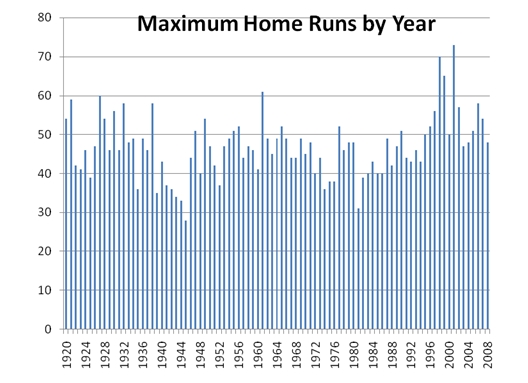
While this is pretty interesting, there is some information that I am interested in that is not immediately obvious from the graphical representation. Specifically, I would like to know the lowest number of home runs, the highest number, the average (or mean), and the standard deviation. In SQL Server, there is a MIN, MAX, AVG, and STDEVP function, but none of them allow expressions that contain aggregates. XLeratorDB allows aggregates to be included, and we can use the QUARTILE function to calculate the MIN and MAX. This saves us a few steps, since we do not need to create a common table expression or a view, and the SQL runs very quickly.
The following SQL will return the data we are looking for:
select wct.QUARTILE_q('select
max(hr)
from batting
where yearid > 1919
group by yearid', 0) as [Min],
wct.QUARTILE_q('select
max(hr)
from batting
where yearid > 1919
group by yearid', 4) as [Max],
wct.AVERAGE_q('select
max(hr)
from batting
where yearid > 1919
group by yearid') as [Average],
wct.STDEVP_Q('select
max(hr)
from batting
where yearid > 1919
group by yearid') as [St. Dev.]
Which returns the following information:
Min Max Average St. Dev.
-------------- -------------- ---------------------- ----------------------
28 73 46.8988764044944 7.91960296334884
(1 row(s) affected)
This means that since 1920, the lowest number of home runs to lead the major leagues was 28 (in 1945) and highest number was 73 (in 2001). The average number of home runs required to lead the league in home runs is almost 47 and the standard deviation is almost 8.
In very general terms, and assuming that the distribution is a ‘normal’ distribution, that means that about 68% (68.2689492%) of the time, we would expect the home run leader for the season to have 47 ± 8 home runs (39–55). A little more than 95% (95.4499736%) of the time, we would expect the home run leader to have approximately 47 ± 16 home runs (31–63).
The STANDARDIZE function will actually show us the number of standard deviations that a particular value represents, which gives us some idea of how the actual performance differences from the hypothetical normal distribution. We can enter the following SQL, which uses a common table expression (just to keep things simple) and the average (mean) and standard deviation from the previous SELECT:
with HR as
(
select yearid,
max(hr) as [Home Runs]
from batting
where yearid > 1919
group by yearid
) select HR.yearid
,wct.STANDARDIZE([Home Runs], 46.8988764044944, 7.91960296334884)
from HR
order by yearid
I then pasted the results into EXCEL and produced the following graph:
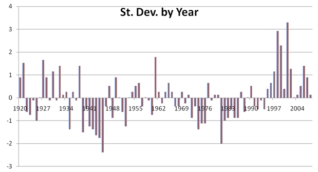
We can immediately see that 2001, with 73 home runs, is more than 3 (3.2958) standard deviations away. In a way, that’s a very interesting number, as in a normal distribution, you expect 99.9% of the results would be within 3.2906 standard deviations. It might be possible to conclude that hitting 73 home runs, purely from this analysis, is not really a statistically significant event. In fact, we have a function, the NORMDIST function, that will tell us the exact probability:
select wct.NORMDIST(73
,46.8988764044944
,7.91960296334884
,0)
Which returns the following information:
----------------------
0.000220568560862717
(1 row(s) affected)
This means that there was a .0221% chance that a result of 73 would be contained in this dataset; in other words, a remote, but not improbable, chance.
There are a couple of additional things that we might want to look at. First, the number of games changed in 1961 from 154 to 162. Second, the 1994 season was shortened by about 50 games. While making those kind of adjustments in a spreadsheet can be tricky and time-consuming, it’s a pretty easy change to the WHERE clause in all of our SELECT statements:
SELECT. . .
where yearid > 1960 and
yearid <> 1994
We would then get the following statistics:
Min Max Average St. Dev.
-------------- -------------- ---------------------- ----------------------
31 73 48.063829787234 8.08835321144887
(1 row(s) affected)
From which we can then produce the following graph:
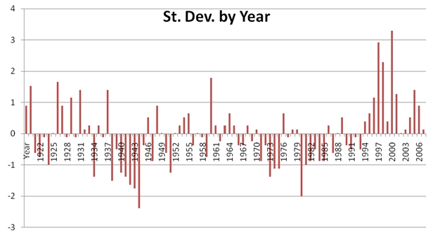
This puts the 2001 season 3.083 standard deviations away, giving it a likelihood of .0426%, slightly less than double the previous calculation.
Earlier in this blog in talking about doing this type of analysis, we assumed that the data represented a normal distribution. There are two measures, SKEW and KURTOSIS that we can use to make that evaluation. And, if you want a good explanation of what a normal distribution is, go here http://en.wikipedia.org/wiki/Normal_distribution.
First, let’s create a different graphical representation of the data by eliminating the time dimension. We are simply going to count the number of times a particular number led MLB in home runs. That graph looks like this:
Visually, we can tell that this isn’t a perfectly normal distribution. The first thing that we will want to measure is the SKEW. We can do this with the following SELECT statement:
select wct.SKEW_q('select
max(hr)
from batting
where yearid > 1919
group by yearid')
Which returns the following results:
----------------------
0.542542382246413
(1 row(s) affected)
A positive value for skewness indicates that a distribution has an asymmetric tail which extends more positive. What this means to me is that normal statistical measures will tend to miss the upside to a greater degree than they miss the downside.
The second measure that we want to look at is KURTOSIS. Again, a simple SELECT statement will give us that information:
select wct.KURT_q('select
max(hr)
from batting
where yearid > 1919
group by yearid')
Which returns the following results:
----------------------
1.14592237200248
(1 row(s) affected)
Kurtosis, like skewness, is a non-dimensional quality. Kurtosis measures the relative peakedness or flatness of a distribution as compared to a normal distribution. Since the kurtosis of this distribution is positive, it is characterized as leptokurtic. One other note, is that the Kurtosis function is identical to the EXCEL KURT function and thus measures excess kurtosis.
Since we know the mean and the standard deviation of the dataset, we can actaully calculate what the normal distriibution would be like. We can create a CTE which gives us every home run value from 28 to 73, and we can then calculate the NORMDIST value for each home run value. We then multilpy that value by 46, which is the range of the values (from 28 to 73). The following SELECT creates that data for us:
with NHR as
(
select 28 as [Home Runs]
UNION ALL
select [Home Runs] + 1
FROM NHR
where [Home Runs] < 73
) select [Home Runs]
,wct.NORMDIST([Home Runs],46.8988764044944,7.91960296334884,0)*46
from NHR
order by 1 option(maxrecursion 46)
Which we can then just paste into EXCEL and graph:
And finally, we can simply plot the actual values against the normalized values and create the following graph:
This provides a visualization of the postive skew and positive kurtosis for the dataset.
In very short order we have been able to perform a pretty sophisticated analysis of this one statistic. I think that this would be quite hard to do in EXCEL and there are almost 100,000 player-seasons that need to be sifted through to get the 89 player-seasons that we are most interested in. That argues very much for putting the data into a database, but SQL Server (and Access), do not have the sophisticated statistical functions which EXCEL provides. XLeratorDB brings those functions into the database and creates a very easy-to-use but powerful environment for doing this kind of analysis.
In this article we have demonstrated a number of statistical functions that can be used to analyze some common statistics. Next week, we will look at a some more baseball statistics and then we will build a simple Monte Carlo simulation, all in SQL Server, for the home run statistic.